Manual Cell Type Annotation Best Practices 2025: A Researcher's Guide to Accurate Single-Cell Analysis
This comprehensive guide provides researchers and drug development professionals with current best practices for manual cell type annotation in single-cell RNA sequencing data.
Manual Cell Type Annotation Best Practices 2025: A Researcher's Guide to Accurate Single-Cell Analysis
Abstract
This comprehensive guide provides researchers and drug development professionals with current best practices for manual cell type annotation in single-cell RNA sequencing data. Covering foundational concepts to advanced validation techniques, we explore how to define cell identities across established types, novel populations, and disease states. The article details systematic workflows from quality control through marker gene validation, addresses common troubleshooting scenarios, and compares manual annotation with emerging automated and AI-assisted methods. With the growing importance of reliable cellular characterization in biomedical research, this resource equips scientists with strategies to produce biologically meaningful and technically sound annotations that withstand scientific scrutiny.
Understanding Cell Identity: The Conceptual Foundation of Manual Annotation
The definition of a cell type, a fundamental concept in biology, has undergone a profound transformation with the advent of single-cell technologies. Traditionally, biologists defined cell types based on morphological characteristics (e.g., the shape of eosinophil granulocytes) and physiological function (e.g., the capacity of stem cells to differentiate) [1]. The introduction of antibody labeling added another dimension, enabling definition via cell surface markers [1]. Today, single-cell RNA sequencing (scRNA-seq) has unlocked the ability to define cell types by their complete gene expression profiles, moving beyond a handful of markers to a holistic, data-driven view of cellular identity [1] [2].
This shift has revealed that cellular properties across different modalities—molecular, morphological, physiological—are highly heterogeneous and do not always align neatly [2]. Consequently, the scientific community actively debates what truly constitutes a cell type, and a single, universal definition remains elusive [1] [2]. This whitepaper, framed within a broader thesis on manual annotation best practices, explores the modern, multi-faceted approach to defining cell type identity. We outline the core principles, detailed methodologies, and essential tools that empower researchers to navigate this complexity and assign meaningful biological identities to the clusters revealed by single-cell transcriptomics.
Modern Frameworks for Cell Type Identity
In the single-cell era, cell identities derived from transcriptomic data generally fall into several interconnected categories, each requiring a slightly different interpretive lens [1].
- Established Cell Types: These are well-characterized populations, such as endothelial cells expressing PECAM1, and are typically straightforward to identify using existing reference datasets and canonical marker genes [1].
- Novel Cell Types: Rare but significant, these are biologically distinct clusters—potentially based on function or developmental origin—that cannot be mapped to known types. Their discovery relies on differential expression analysis and must be followed by functional validation [1].
- Cell States and Disease Stages: scRNA-seq can capture transient, dynamic conditions such as activation, stress, or pathology. These are not necessarily distinct cell types but rather functional or disease-associated alterations within a type [1].
- Developmental Stages: In developmental contexts, cells exist on a continuum. Trajectory inference and pseudotime analysis are used to reconstruct these paths and annotate cells according to their position in a differentiation process [1].
Foundational Pillars of Cell Type Annotation
Robust cell type annotation rests on three foundational pillars, which are often applied in an iterative manner.
Pillar 1: In-depth Preprocessing and Quality Control High-quality annotation is impossible without high-quality data. The foundation is rigorous quality control to filter out low-quality cells, doublet detection to exclude multiplets, and batch effect correction to mitigate technical variation [1] [3] [4]. This process concludes with preliminary clustering to group cells with similar transcriptomic profiles, providing the initial structure for annotation [1]. For example, best practices for 10x Genomics data include filtering cells based on UMI counts, the number of genes detected, and the percentage of mitochondrial reads to remove unhealthy cells or ambient RNA contamination [4].
Pillar 2: Reference-Based Annotation This approach involves aligning the gene expression profiles of cell clusters to well-annotated reference datasets or cell atlases, such as those provided by the Human Cell Atlas or the BRAIN Initiative Cell Census Network [1] [2]. Tools like SingleR and Azimuth perform this mapping computationally [1] [5]. A key advantage is that references like Azimuth provide annotations at different levels of granularity, allowing researchers to choose the resolution that best fits their biological question [1].
Pillar 3: Expert-Guided Manual Refinement Automated methods, while powerful, can miss subtle distinctions or be misled by ambiguous expression patterns [1]. Manual refinement adds a crucial layer of biological insight by:
- Verifying expression of canonical marker genes.
- Interpreting results from differential gene expression analysis.
- Contextualizing findings within the scientific literature.
- Integrating the researcher's domain-specific knowledge to resolve edge cases and identify novel populations [1].
This collaborative process between computational output and expert intuition ensures that final cell type assignments are both technically sound and biologically meaningful [1].
Quantitative Comparison of Annotation Tools and Performance
The field has developed a diverse array of computational tools to assist with cell type annotation. They can be broadly categorized as reference-based, marker-based, or hybrid methods, each with distinct strengths and performance characteristics.
Table 1: Classification and Characteristics of Selected Cell Type Annotation Tools
| Tool Name | Category | Core Methodology | Key Features |
|---|---|---|---|
| SingleR [5] [6] | Reference-based | Spearman correlation to reference scRNA-seq data | Fast, does not require clustering; depends on reference quality. |
| ScType [5] [6] | Marker-based | Scoring system using positive and negative marker sets | Utilizes comprehensive marker database (ScTypeDB); supports negative markers. |
| ScInfeR [6] | Hybrid | Graph-based integration of references and marker sets | Hierarchical framework for subtype identification; versatile across scRNA-seq, scATAC-seq, and spatial omics. |
| Garnett [6] | Marker-based | Generalized linear machine learning model | Performs hierarchical classification of types and subtypes; depends on training data quality. |
| LICT [7] | LLM-based | Multi-model LLM integration with "talk-to-machine" strategy | Reference-free; provides objective credibility evaluation of annotations. |
| GPTCelltype [5] | LLM-based | Leverages GPT-4's language understanding with marker gene input | No custom reference needed; cost-effective; can annotate with high granularity. |
Recent benchmarks have quantitatively evaluated the performance of these tools, including emerging methods that leverage large language models (LLMs).
Table 2: Performance Benchmarking of Annotation Tools Across Diverse Datasets
| Tool / Method | Reported Agreement with Manual Annotation | Notable Strengths | Noted Limitations |
|---|---|---|---|
| GPT-4 (via GPTCelltype) [5] | Over 75% full or partial match in most tissues/types. | High accuracy across many tissues; cost-efficient; requires no custom reference. | Performance dips for small populations (<10 cells); cannot annotate malignant cells without distinct gene sets. |
| LICT [7] | Significantly reduced mismatch rates (e.g., 9.7% vs. 21.5% in PBMCs). | Superior in low-heterogeneity datasets; provides objective reliability score. | Over 50% inconsistency remains for some low-heterogeneity data. |
| ScInfeR [6] | Superior performance in >100 cell-type prediction tasks. | Robust to batch effects; versatile across data modalities (RNA, ATAC, spatial). | Dependency on the quality of integrated references and marker sets. |
Detailed Experimental Protocols for Cell Type Annotation
A Standardized Workflow for scRNA-seq Cell Type Annotation
The following protocol describes a comprehensive combinatorial approach, integrating both reference-based and manual methods for robust annotation [1].
Step 1: Data Preprocessing and Clustering
- Quality Control: Filter cells based on metrics like UMI counts, genes detected, and mitochondrial read percentage. For PBMCs, a common threshold is to remove cells with >10% mitochondrial UMIs [4].
- Normalization and Scaling: Normalize the gene expression matrix for sequencing depth and scale the data.
- Dimensionality Reduction and Clustering: Perform principal component analysis (PCA), followed by graph-based clustering and visualization with UMAP or t-SNE to reveal the cellular population structure [1].
Step 2: Obtain Preliminary Annotations via Reference Mapping
- Reference Selection: Identify a suitable, well-annotated reference dataset (e.g., from the Human Cell Atlas or Azimuth) that matches the tissue and species of interest [1].
- Automated Label Transfer: Use a tool like SingleR or the Azimuth web application to map your clusters against the reference. This will generate a preliminary cell type label for each cluster [1] [5].
Step 3: Expert-Driven Manual Refinement and Validation
- Differential Expression Analysis: For each cluster, identify the top marker genes using a statistical test like the two-sided Wilcoxon rank-sum test [1] [5].
- Interrogate Marker Gene Expression: Create visualizations (dot plots, feature plots, violin plots) to inspect the expression of known canonical markers for the proposed cell types, as well as the top differentially expressed genes from your analysis.
- Contextualize and Refine: Compare the automated labels with the marker evidence. For example, if a cluster is labeled "Stromal Cells" but expresses high levels of type I collagen genes (COL1A1, COL1A2) and not type II, it may be more accurately annotated as "Fibroblasts" [5]. Use this evidence to accept, refine, or reject the automated labels.
Step 4: Finalize and Document
- Produce a final annotated UMAP plot and document the evidence (reference source, key marker genes, differential expression results) used for each cell type's identity to ensure reproducibility.
Protocol for LLM-Assisted Annotation with GPTCelltype
The emergence of LLMs like GPT-4 offers a powerful, reference-free alternative. The following protocol has been validated across hundreds of cell types [5].
- Input Preparation: For the cell cluster of interest, generate a list of marker genes. Benchmarking indicates that using the top 10 differential genes identified by the two-sided Wilcoxon test yields optimal performance with GPT-4 [5].
- Prompting the Model: Use a basic prompt strategy to query the model. An example prompt structure is: "What is the most specific cell type identity given the expression of the following marker genes: [list of top 10 genes]?" [5].
- Validation and Iteration: The model's output should be treated as a hypothesis. Crucially, validate the annotation by checking the expression of known marker genes for the proposed cell type in your dataset. For ambiguous cases, the "talk-to-machine" strategy implemented in LICT can be used: the model is provided with the validation results and asked to refine its annotation [7].
Visualizing Annotation Workflows and Data Integration
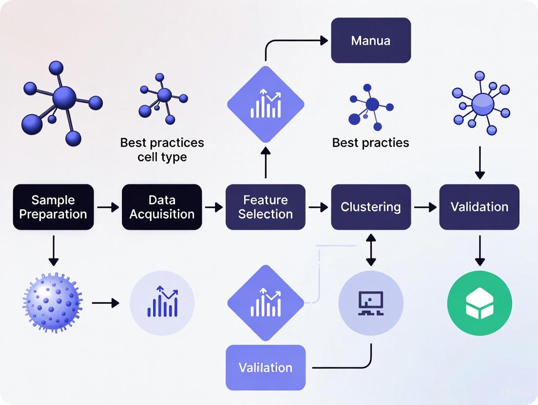
The following diagram illustrates the core logical workflow for modern cell type annotation, integrating both traditional and AI-assisted methods.
Figure 1: Integrated Cell Type Annotation Workflow. This diagram outlines the key steps in a modern annotation pipeline, from raw data to a finalized annotated dataset, highlighting the complementary roles of automated tools and expert-led refinement.
A critical prerequisite for multi-sample annotation is the integration of datasets to remove technical batch effects. The following diagram visualizes the semi-supervised integration process used by tools like STACAS, which leverages prior cell type knowledge to preserve biological variance.
Figure 2: Semi-Supervised Data Integration. This process uses prior cell type labels to guide the integration of multiple datasets, ensuring that technical batch effects are removed without obscuring true biological differences.
Successful cell type annotation relies on a suite of computational tools, reference data, and databases. The following table details key resources.
Table 3: Essential Reagents and Resources for Cell Type Annotation
| Resource Name | Type | Primary Function in Annotation | Key Application Notes |
|---|---|---|---|
| Seurat [8] | R Toolkit | Comprehensive environment for single-cell data analysis, including preprocessing, integration, and clustering. | The de facto standard for many analysis workflows; provides functions for reference-based integration. |
| Cell Ranger [4] | Analysis Pipeline | Processes raw 10x Genomics FASTQ data into gene-cell count matrices and performs initial secondary analysis. | Generates the foundational data (count matrices) for all downstream annotation work. |
| Human Cell Atlas [2] | Reference Database | Aims to create comprehensive reference maps of all human cells. | A growing source of high-quality, standardized reference data for multiple tissues. |
| ScInfeRDB [6] | Marker Database | An interactive database of 2,497 manually curated gene markers for 329 cell types across 28 tissues. | Can be directly integrated with the ScInfeR tool for marker-based annotation. |
| CellMarker / PanglaoDB [6] | Marker Database | Databases of cell type-specific markers compiled from literature. | Useful for manual refinement and validation of cluster identities. |
| Azimuth [1] [5] | Web Application / Reference | Provides automated cell type annotation for user-uploaded data against curated reference atlases. | Offers annotations at multiple levels of resolution, from broad categories to fine subtypes. |
The journey to define cell type identity has evolved from relying on simple morphological observations to integrating complex, high-dimensional transcriptomic data. The modern paradigm is combinatorial, leveraging automated reference mapping, emerging AI and LLM-based tools, and, indispensably, expert-guided manual refinement [1] [7] [5]. This integrated approach ensures that annotations are not only computationally derived but also biologically grounded.
Looking forward, several trends will shape the future of cell type annotation. The field is moving towards a multi-omic definition of cell identity, integrating not just transcriptomics but also epigenomic (e.g., scATAC-seq), proteomic, and spatial data to build a more complete picture [2] [6]. Furthermore, as LLM-based tools mature, their ability to interpret complex biological contexts will improve, but they will likely remain most powerful when used in a "human-in-the-loop" model [7]. Finally, the success of any annotation effort hinges on the quality of the underlying data and the availability of comprehensive, tissue-specific reference atlases. Continued community efforts to build and standardize these resources, such as the Human Cell Atlas, will be critical for deepening our understanding of cellular function in health and disease [1] [2].
In the era of single-cell biology, the definition of cell type identity is continuously evolving, moving beyond traditional morphological and physiological descriptions to encompass detailed transcriptomic signatures [1]. Assigning cell type identities is a central challenge in interpreting single-cell RNA sequencing (scRNA-seq) data, transforming clusters of gene expression data into meaningful biological insights. This process is fundamental for understanding complex biological systems, disease mechanisms, and developmental processes [1] [9]. Robust cell type identification depends on multiple factors: data quality, availability of suitable reference studies, and the validity of chosen marker genes or gene sets [1]. The annotation process is highly collaborative, combining computational expertise with deep biological knowledge to ensure annotations are technically sound and biologically meaningful [1]. Within this framework, cellular identities generally fall into several distinct categories, each requiring specific approaches for identification and validation.
Established Cell Types
Established cell types are the most straightforward to identify and are typically recognized through comparison with existing reference datasets or canonical marker genes [1]. These cell types have consistent, well-documented transcriptomic profiles supported by extensive previous research.
- Identification Methodology: The primary method for identifying established cell types is reference-based annotation. This involves aligning the gene expression profiles of single cells against established reference datasets from similar tissues using tools such as SingleR or Azimuth [1] [9]. The Azimuth project, for instance, provides annotations at different levels of granularity, from broad categories to detailed subtypes [1].
- Marker Gene Verification: Many established cell types possess distinct marker genes. For example, PECAM1 is a classic marker for endothelial cells, and PFN1 for osteocytes [1]. Verification involves checking for the expression of these canonical markers in the clusters of interest.
- Validation and Refinement: After an initial automated annotation, results are checked for consistency. If a reference indicates two clusters represent the same established cell type, they are merged. If it suggests finer distinctions, the clustering resolution is adjusted to capture those subtypes [1].
Novel Cell Populations
Novel cell populations are biologically distinct clusters that do not align with any known cell type based on existing references or marker gene databases. Their identification is a key driver of discovery in single-cell research.
- Identification Methodology: The process begins with differential expression analysis, which identifies genes that are statistically significantly upregulated in a cluster of interest compared to all other clusters [1] [9]. A cluster is considered potentially novel if its top differentially expressed genes do not match any known cell type signature.
- Biological Distinctness Assessment: Researchers must then assess whether the cluster's distinct transcriptomic profile correlates with a unique function or developmental origin [1]. This requires careful literature review and domain expertise to argue for the existence of a new cell type.
- Functional Validation: The identification of a novel cell type is considered provisional until followed up with independent validation experiments. This may include fluorescence in situ hybridization (FISH) to confirm spatial localization, or functional assays to determine the cell's role [1].
Transitional States and Disease-Associated Phenotypes
Cells can undergo changes in state without transitioning to a completely different type. These transitional states are often linked to processes like activation, stress, or disease pathology.
- Identification Methodology: Tools like gene set enrichment analysis or co-expression analysis are used to identify transcriptomic patterns associated with specific cellular states, such as activation or apoptosis [1]. In disease research, this involves comparing cells from healthy and diseased tissues to identify disease-associated expression signatures.
- Contextual Interpretation: Identifying a cell state requires deep biological context. For example, an increased level of mitochondrial transcripts can indicate an unhealthy or stressed cell state [4]. However, for some cell types like cardiomyocytes, mitochondrial gene expression is biologically meaningful and should not be used as a stress indicator [4].
- Trajectory Analysis: For understanding progressive changes, such as in development or disease progression, trajectory inference and pseudotime analysis are employed. These tools reconstruct the paths cells take as they progress from one state to another, providing dynamic insights beyond static classification [1].
Quantitative Comparison of Cell Type Annotation Methodologies
The choice of methodology for assigning cellular identities has a significant impact on the accuracy and reliability of the results. The following table summarizes the key approaches, their mechanisms, and their performance characteristics.
Table 1: Comparison of Cell Type Annotation Methodologies
| Method Category | Examples | Core Mechanism | Relative Speed | Key Requirements | Pros | Cons |
|---|---|---|---|---|---|---|
| Manual Curation | N/A | Inspection of cluster-specific differential genes against known markers [9]. | Slow | Known marker genes, accurate clustering, literature/databases (e.g., CellMarker) [9]. | Complete expert control; high reliability if meticulous [9]. | Time-consuming; requires expert knowledge; public databases not always updated [9]. |
| Traditional Automated | SingleR, CellTypist, Azimuth [9] [5] | Classification or reference mapping of cells to a reference dataset [9]. | Fast [5] | A single high-quality reference dataset similar to the query [9]. | Fast; no clustering needed; reliable with a good reference [9]. | Matching reference not always available; custom reference creation is non-trivial [9]. |
| AI and Foundation Models | scGPT, SCimilarity, Geneformer [9] [5] [10] | Leveraging models pre-trained on millions of cells to annotate using marker gene inputs [5]. | Varies (can be fast) [9] | GPU resources for some; possible fine-tuning with a reference [9]. | Can work without a reference; integrates multiple references in one model [9]. | Difficult setup; models are "black boxes" and not frequently updated [9]. |
| Knowledgebase-Driven | CellKb [9] | Rank-based search against a manually curated database of cell type signatures from literature [9]. | Fast | Web access; selection of relevant references from the knowledgebase [9]. | No installation; uses multiple, regularly updated references; simple interface [9]. | Not a free service [9]. |
Performance Note: A recent evaluation of GPT-4 found it could generate cell type annotations that fully or partially matched manual annotations in over 75% of cell types across several datasets, showcasing the potential of advanced AI in this field [5].
Integrated Experimental Workflow for Cell Type Annotation
A robust cell type annotation pipeline integrates multiple steps, from raw data processing to final validation. The following workflow diagram and protocol outline this integrated process.
Diagram: Integrated Workflow for Cell Identity Annotation
Detailed Protocol for Cell Identity Classification
In-depth Preprocessing and Quality Control:
- Quality Control: Filter out low-quality cells based on metrics like total UMI counts, number of features (genes), and the percentage of mitochondrial reads. For example, in PBMC data, a threshold of 10% mitochondrial reads is often used to remove damaged cells [4].
- Batch Correction: Apply computational methods to mitigate technical variation caused by differences in sample preparation or sequencing runs [1].
- Clustering: Perform a preliminary clustering analysis to group cells with similar transcriptomic profiles, providing the initial structural view of the dataset [1].
Combinatorial Annotation Strategy:
- Reference-Based Mapping: Use tools like Azimuth to map your pre-processed dataset against established reference atlases. This provides a first, automated preliminary annotation [1].
- Differential Expression: For each cluster, perform differential expression analysis (e.g., using a two-sided Wilcoxon rank-sum test) to identify genes that are statistically significantly upregulated compared to all other cells. The top genes (e.g., top 10) form the marker gene signature for the cluster [5].
- Marker Gene Cross-Referencing: Cross-reference the differential gene lists with canonical marker genes from literature and databases. This step is crucial for verifying established types and identifying the hallmarks of novel populations or states [1] [9].
Expert-Led Refinement and Validation:
- Cluster Merging/Splitting: Based on the annotation results, iteratively refine the clusters. Merge clusters predicted to be the same type or increase resolution to separate subtypes [1].
- Contextual Interpretation: Integrate client or domain-specific knowledge to interpret ambiguous clusters, edge cases, and biologically plausible states [1].
- Independent Validation: Plan and execute follow-up experiments of another nature (e.g., immunohistochemistry, functional assays) to further characterize the identified cell types, especially novel ones [1].
Successful cell type annotation relies on a suite of computational tools, reference data, and experimental reagents.
Table 2: Key Research Reagent Solutions for scRNA-seq Annotation
| Tool/Reagent Category | Examples | Primary Function |
|---|---|---|
| Commercial Platforms & Software | 10x Genomics Cell Ranger, Loupe Browser [4] | Processes raw sequencing data (FASTQ) into gene-cell matrices; provides initial QC, clustering, and interactive data visualization [4]. |
| Reference Datasets & Atlases | HuBMAP, Azimuth, Tabula Sapiens, Human Cell Atlas [1] [5] | Serve as a ground truth for reference-based annotation, providing pre-annotated cell types from various tissues [1]. |
| Automated Annotation Tools | SingleR, CellTypist, scGPT [9] [5] | Provide algorithmic cell type prediction using classification or reference mapping, reducing manual effort [9] [5]. |
| Marker Gene Databases | CellKb, CellMarker, PanglaoDB [9] | Curated collections of cell type-specific marker genes from published literature, used for manual verification of cluster identities [9]. |
| Experimental Validation Reagents | Antibodies for IHC/FISH, CRISPR kits [1] | Used for independent validation of cell type identities and functions identified through scRNA-seq analysis [1]. |
Assigning cell type identities is a central challenge and a foundational step in interpreting single-cell data. It is the process of transforming clusters of gene expression data into clear, meaningful biological insights [1]. Fundamentally, there is no universal method for defining cell identity [1]. With every publication, researchers must propose a cell type label and deliver compelling arguments for their labeling by extracting evidence from scRNA-seq data, informing scientific literature, and performing validation experiments [1]. This process is highly collaborative and not merely a default part of preliminary analysis; it requires partnering computational expertise with deep domain-specific biological knowledge to ensure annotations are both technically sound and biologically meaningful [1].
The following diagram illustrates the core decision-making workflow in manual cell type annotation, highlighting the critical role of researcher expertise at each stage.
The Inherent Complexities of Cell Identity
The very definition of a "cell type" is actively debated and continuously evolving, moving beyond traditional definitions based on morphology and physiology to encompass gene expression profiles and molecular states [1]. This complexity means cell identities often fall into multiple, sometimes overlapping, categories:
- Established cell types are identified through reference datasets and distinct markers (e.g., PECAM1 for endothelial cells) [1].
- Novel cell types are discovered when clusters are biologically distinct based on function or developmental origin, guided by differential expression and functional validation [1].
- Cell states and disease stages represent transient changes in response to perturbation, identified through patterns tied to activation, stress, or pathology [1].
- Developmental stages reveal progression from progenitor to mature cell types, reconstructed using trajectory and pseudotime analyses [1].
Methodological Landscape: From Manual Curation to AI Assistance
Traditional and Emerging Annotation Approaches
Cell type annotation methodologies generally fall into three categories, each with distinct strengths and limitations, as summarized in the table below.
Table 1: Comparison of Cell Type Annotation Methodologies
| Method Category | Key Examples | Pros | Cons | Expertise Dependency |
|---|---|---|---|---|
| Manual Annotation | Marker gene checking with databases (CellMarker, PanglaoDB) [9] | Complete control; High reliability if meticulous [9] | Time-consuming; Requires known markers; Depends on accurate clustering [9] | Very High |
| Automated Reference-Based | SingleR, Azimuth, CellTypist, scmap [9] [11] | Fast; No clustering needed; Objective [9] | Requires high-quality matching reference; Limited customization [9] | Medium |
| AI & Foundation Models | LICT, scGPT, Geneformer, Scimilarity [7] [9] | Can work without reference; Integrated multiple references [9] | Difficult setup; Models infrequently updated; Struggles with rare cell types [9] | Medium to High |
The Promise and Limitations of AI-Based Tools
Recent advancements have introduced artificial intelligence (AI) and large language models (LLMs) to cell type annotation. Tools like LICT (LLM-based Identifier for Cell Types) leverage a "talk-to-machine" strategy, where the model is iteratively queried with marker gene expression patterns to refine its predictions [7]. While these tools can reduce mismatch rates in highly heterogeneous datasets like PBMCs from 21.5% to 9.7% compared to earlier methods [7], their performance diminishes with less heterogeneous datasets. For example, even top-performing LLMs like Gemini 1.5 Pro and Claude 3 achieve only 39.4% and 33.3% consistency with manual annotations for human embryo and stromal cell data, respectively [7]. This highlights that AI tools serve as aids rather than replacements for expert judgment, particularly in complex or novel biological contexts.
Quantitative Benchmarks: How Methods Compare
Performance Across Dataset Types
Rigorous benchmarking studies provide quantitative evidence of the challenges in automated annotation. The following table summarizes the performance of a leading LLM-based method (LICT) across diverse biological contexts, demonstrating the variability in annotation success.
Table 2: Performance of LICT (LLM-based method) Across Diverse Biological Contexts [7]
| Dataset Type | Example Tissue/Condition | Match Rate with Manual Annotation | Key Challenges |
|---|---|---|---|
| High Heterogeneity | Peripheral Blood Mononuclear Cells (PBMCs) [7] | 90.3% (Low mismatch rate of 9.7%) [7] | Distinguishing closely related immune subtypes |
| High Heterogeneity | Gastric Cancer [7] | 91.7% (Low mismatch rate of 8.3%) [7] | Separating malignant from non-malignant cells |
| Low Heterogeneity | Human Embryos [7] | 48.5% (Match rate) [7] | Limited transcriptomic diversity between early lineages |
| Low Heterogeneity | Mouse Stromal Cells [7] | 43.8% (Match rate) [7] | Subtle differences between fibroblast subtypes |
Spatial Transcriptomics Present Unique Hurdles
In spatial transcriptomics, the challenge intensifies. A 2025 benchmarking study on 10x Xenium data for human HER2+ breast cancer found that reference-based methods like SingleR, while performing best among automated tools, still required manual validation, particularly for rare or ambiguous cell populations [11]. The study emphasized that manual annotation based on marker genes, despite being time-consuming, remains crucial for reconciling discrepancies and ensuring biologically plausible results [11].
A Practical Protocol for Manual Annotation
This section provides a detailed, executable protocol for researchers performing manual cell type annotation, incorporating both reference-based and expert-driven refinement.
Foundational Preprocessing and QC
- Step 1: Rigorous Quality Control - Filter out low-quality cells or genes and exclude multiplets. Critically assess metrics like percentage of mitochondrial reads, which can indicate stressed or dying cells (e.g., use <10% mt reads as a threshold for PBMCs) [4].
- Step 2: Batch Effect Correction - Apply bioinformatic corrections to mitigate technical variation from differences in sample preparation or sequencing runs [1].
- Step 3: Preliminary Clustering - Perform clustering analysis to group cells with similar transcriptomic profiles, providing the initial structural view of the dataset [1]. Use UMAP or t-SNE for visualization.
Reference-Based Annotation
- Step 4: Literature and Atlas Review - Conduct an in-depth review to identify suitable reference datasets and canonical marker genes for the expected cell types in the tissue of interest [1].
- Step 5: Automated Label Transfer - Use tools like SingleR or Azimuth to align gene expression profiles of each cell with chosen references. These tools provide annotations at different levels, from broad categories to detailed subtypes [1].
- Step 6: Iterative Cluster Refinement - Check how predicted cell types align with clusters. Merge clusters predicted to be the same type or adjust clustering resolution to capture finer differences. Use multiple references to generate a robust consensus annotation [1].
The Crucial Manual Refinement Cycle
- Step 7: Differential Expression Analysis - For each cluster, identify statistically significant upregulated genes compared to all other clusters. This generates cluster-specific gene lists beyond the preliminary markers [9].
- Step 8: Canonical Marker Validation - Manually check the expression patterns of known canonical marker genes for the hypothesized cell type. Use databases like CellMarker or PanglaoDB, but be aware they are not always regularly updated [9].
- Step 9: Biological Contextualization - Integrate domain knowledge to interpret ambiguous clusters or edge cases. This is often essential for distinguishing closely related cell subtypes, identifying transitional states, or flagging potentially novel populations [1].
- Step 10: Resolution of Inconsistencies - Reconcile discrepancies between reference-based predictions, marker gene evidence, and biological plausibility. This may involve re-clustering, consulting additional literature, or hypothesizing new cell states [1].
The following diagram details the iterative "talk-to-machine" strategy, a modern approach that exemplifies the collaboration between computational tools and researcher expertise.
Table 3: Key Research Reagent Solutions for Cell Type Annotation
| Tool/Resource | Function in Annotation | Application Context |
|---|---|---|
| CellKb [9] | A knowledgebase of high-quality cell type signatures from manually curated publications; allows use of multiple references without integration. | Annotating individual cells or clusters via a web interface without installation. |
| CellMarker/PanglaoDB [9] | Databases of known marker genes for various cell types across tissues and species. | Initial hypothesis generation during manual refinement and marker validation. |
| Azimuth [1] [11] | A reference-based annotation tool integrated within the Seurat platform; provides annotations at different resolution levels. | Transferring labels from a prepared reference (e.g., from the Human Cell Atlas) to query data. |
| SingleR [11] | A reference-based method that predicts cell types using correlation between query and reference datasets. | Fast, accurate annotation of common cell types, particularly in immune cells [11]. |
| LICT [7] | An LLM-based tool that uses a "talk-to-machine" approach for reference-free annotation. | Generating initial labels when a high-quality reference is unavailable; providing an objective credibility score. |
| STAMapper [12] | A heterogeneous graph neural network for transferring labels from scRNA-seq to single-cell spatial transcriptomics data. | Annotating challenging spatial data with high accuracy, especially with low gene numbers. |
Robust cell type identification is not a solved computational problem but a complex inference process that depends on multiple factors: data quality, the availability of suitable references, and the biological validity of chosen markers [1]. While automated and AI-driven methods are becoming increasingly powerful, they do not obviate the need for deep biological expertise. Instead, they shift the researcher's role from performing tedious comparisons to exercising critical judgment in interpreting results, reconciling discrepancies, and applying contextual knowledge [7] [9].
The most reliable annotations emerge from a combinatorial approach that integrates computational predictions with expert curation. It is also a critical best practice to follow up scRNA-seq experiments with independent validation using other methodological approaches, such as fluorescence in situ hybridization or immunohistochemistry, to further characterize the cells in a sample and confirm their identity [1]. Ultimately, accurately naming a cell type is the first step toward understanding its function, and this process remains fundamentally a human interpretation of complex data within a biological context.
In single-cell RNA sequencing (scRNA-seq) research, the path to biologically meaningful discoveries is paved long before the assignment of cell type labels. Manual cell type annotation, a cornerstone of biological interpretation, is entirely dependent on the quality of the data and the integrity of the initial clustering upon which it is built [1]. This guide details the two key prerequisites for any rigorous annotation workflow: comprehensive data quality assessment (DQA) and a foundational understanding of clustering analysis. Without excellence in these initial stages, even the most sophisticated annotation tools and expert biological knowledge can lead to spurious conclusions. The process transforms raw data into clusters of cells with similar expression profiles, which are then interpreted and labeled by researchers [1]. This document, framed within a broader thesis on manual cell type annotation best practices, provides researchers and drug development professionals with the essential technical groundwork to ensure their analytical pipeline is robust, reproducible, and ready for accurate biological interpretation.
Data Quality Assessment: Ensuring Analytical Robustness
A rigorous Data Quality Assessment (DQA) is the first and most critical step in the scRNA-seq pipeline. It serves to identify and mitigate technical artifacts that can obscure true biological signal, ensuring that downstream clustering and annotation are based on reliable data.
Core Quality Control Metrics and Filtering Strategies
After processing raw sequencing data with pipelines like Cell Ranger, the initial DQA involves examining key metrics to make informed decisions about filtering out low-quality cells [4]. The standard approach involves diagnosing three primary metrics for each cell barcode, which help distinguish intact cells from background noise or damaged cells.
Table 1: Key Quality Control Metrics for Single-Cell RNA-seq Data
| Metric | Description | Interpretation & Common Thresholds |
|---|---|---|
| UMI Counts per Cell | Total number of Unique Molecular Identifiers (UMIs) detected per cell. | Indicates sequencing depth. Cells with very high counts may be multiplets; cells with very low counts may be empty droplets or contain ambient RNA [4]. |
| Genes Detected per Cell | The number of unique genes detected per cell. | Correlates with UMI counts. High numbers can indicate multiplets; low numbers can indicate poor-quality cells or empty droplets [4]. |
| Mitochondrial Read Fraction | The percentage of reads mapping to the mitochondrial genome. | A high percentage (>10% in PBMCs) often indicates apoptotic or stressed cells due to cytoplasmic mRNA leakage [4]. |
These diagnostics are visualized and used for manual filtering in tools like Loupe Browser, where distributions are examined to remove extreme outliers [4]. Furthermore, the HTML summary file generated by Cell Ranger provides an initial, critical overview, indicating whether "No critical issues were identified" and showing expected values for cells recovered, mapping rates, and median genes per cell [4].
Addressing Technical Noise and Batch Effects
Beyond per-cell filtering, DQA must account for broader technical noise. A key challenge is ambient RNA, which arises from free-floating RNA released by lysed cells during sample preparation. This contamination can mask true expression patterns, particularly for rare cell types. Computational tools like SoupX and CellBender are recommended to estimate and subtract this background signal [4]. Additionally, when multiple samples or batches are involved, batch effect correction is a vital pre-processing step to prevent technical variation from being misinterpreted as biological variation during clustering [1]. This ensures that cells cluster together based on their type or state, not their sample of origin.
Clustering Analysis Fundamentals: Grouping Cells by Similarity
Clustering is the unsupervised learning process that groups cells based on the similarities in their gene expression profiles, forming the structural basis upon which cell type identities are assigned [13] [1].
The Clustering Workflow and Algorithm Selection
The standard clustering workflow in scRNA-seq analysis involves a sequence of steps designed to reduce dimensionality and identify natural groupings within the data. The following diagram illustrates this foundational workflow and its direct connection to the subsequent manual annotation phase.
The choice of clustering algorithm can significantly impact the results. Below is a comparison of common algorithms used in single-cell analysis, each with distinct strengths and limitations.
Table 2: Comparison of Common Clustering Algorithms in Single-Cell Analysis
| Algorithm | Underlying Principle | Advantages | Disadvantages |
|---|---|---|---|
| K-means [14] | Partitional; minimizes variance within K pre-defined clusters. | Computationally efficient for large datasets. | Requires prior specification of K (number of clusters); assumes spherical clusters. |
| Hierarchical Clustering [13] [14] | Builds a tree-like structure (dendrogram) of clusters. | Does not require pre-specifying cluster count; highly interpretable. | Computationally intensive on large datasets; sensitive to noise. |
| Leiden Algorithm [15] | Optimizes network structure to find tightly connected communities. | Fast, scalable, and guarantees connected clusters. | Resolution parameter impacts granularity; may require tuning. |
| DBSCAN [14] | Density-based; identifies dense regions separated by sparse areas. | Can find arbitrarily shaped clusters and identify outliers/noise. | Struggles with clusters of varying densities. |
In modern single-cell pipelines, such as those implemented in Scanpy, the Leiden algorithm (a successor to the Louvain method) is frequently used for community detection in graphs built from cells in a reduced dimensionality space [15].
Determining Cluster Resolution and Validation
A crucial step after clustering is validation to ensure the groups are robust and meaningful. Using metrics like the silhouette score or the Davies-Bouldin index provides a quantitative measure of clustering quality, indicating how well-separated the clusters are [14]. Furthermore, the choice of resolution is paramount. A too-low resolution may merge distinct cell types, while a too-high resolution may split a single cell type into multiple, overly fine-grained clusters. This is often an iterative process, guided by biological knowledge and the use of differential expression analysis to test for distinct transcriptomic profiles between clusters [1] [15].
The Scientist's Toolkit: Essential Research Reagents and Computational Tools
A successful single-cell study relies on a combination of wet-lab reagents and dry-lab computational tools. The table below details key resources essential for generating and analyzing data for manual cell type annotation.
Table 3: Essential Toolkit for Single-Cell RNA-seq Analysis
| Item / Tool | Type | Primary Function |
|---|---|---|
| Chromium Platform & Kits (e.g., 3' Gene Expression v4) [4] | Wet-lab Reagent | Platform for generating barcoded single-cell RNA-seq libraries from cell suspensions. |
| Cell Ranger [4] | Computational Tool | Primary analysis pipeline that processes FASTQ files to perform alignment, barcode counting, and initial clustering. |
| Loupe Browser [4] | Computational Tool | Interactive desktop software for visualization, quality control (filtering by UMI, genes, mt-reads), and initial exploration of clustering results. |
| Seurat / Scanpy [1] [15] | Computational Tool | Comprehensive R/Python packages for the entire downstream analysis workflow, including advanced normalization, dimensionality reduction, clustering, and differential expression. |
| Reference Atlases (e.g., Human Cell Atlas) [1] | Data Resource | Curated collections of cell type gene expression profiles used for automated (e.g., via Azimuth) or manual reference-based annotation. |
| Ambient RNA Removal Tools (e.g., SoupX, CellBender) [4] | Computational Tool | Algorithms to correct for background contamination, enhancing the signal-to-noise ratio in the count matrix. |
Integrated Workflow: From Raw Data to Annotated Clusters
The individual components of DQA and clustering form a cohesive, sequential pipeline. The following diagram provides a high-level overview of the complete journey from raw sequencing data to annotated cell types, highlighting the critical prerequisites covered in this guide.
The reliability of manual cell type annotation is inextricably linked to the meticulous application of data quality assessment and clustering analysis fundamentals. As the field advances with new technologies like single-cell long-read sequencing and automated annotation tools powered by large language models, the demand for high-quality input data and robust clustering only increases [10] [15]. By establishing a rigorous, reproducible approach to these foundational steps, researchers ensure that their subsequent biological interpretations and conclusions about cell identity, state, and function are built upon a solid analytical foundation, ultimately driving meaningful discoveries in biology and drug development.
Cell type annotation, a foundational step in single-cell RNA sequencing (scRNA-seq) analysis, has evolved from a purely manual, expert-driven process to one increasingly assisted by sophisticated computational tools. However, the integration of computational output with domain-specific biological knowledge remains a critical component for achieving accurate, biologically meaningful, and reproducible results. This whitepaper delineates the best practices for this collaborative paradigm, framing it within the broader context of manual annotation as the gold standard. It provides a technical guide for researchers and drug development professionals on effectively marrying automated predictions with expert curation to navigate the complexities of cellular heterogeneity, novel cell state discovery, and the inherent challenges of transcriptomic data interpretation.
The Indispensable Role of Manual Annotation and the Case for Collaboration
Manual cell type annotation is traditionally regarded as the benchmark for quality in scRNA-seq analysis. This process involves clustering cells based on gene expression profiles and then assigning cell identities by meticulously comparing cluster-specific gene lists with known canonical markers from scientific literature and databases [1] [16]. This expert-dependent approach provides deep biological insights and allows for the identification of novel or transient cell states that may not be predefined in existing classification schemas.
However, the manual process is labor-intensive, time-consuming, and suffers from poor scalability as datasets grow to encompass millions of cells [9] [17]. It is also susceptible to subjective biases and requires continuous consultation of a vast and ever-expanding body of literature. These limitations have spurred the development of numerous automated annotation methods. The core thesis of this guide is that these computational methods are not replacements for expert knowledge but are powerful partners. The most robust annotation strategy is a collaborative, iterative cycle where computational tools generate initial hypotheses and experts refine, validate, or correct these predictions using their domain-specific knowledge [1]. This synergy mitigates the weaknesses of both approaches, enhancing both efficiency and biological fidelity.
A Landscape of Computational Annotation Methods
Automated cell type annotation methods can be broadly categorized, each with distinct strengths, weaknesses, and appropriate use cases. Understanding this landscape is the first step toward effective integration.
Table 1: Categorization of Automated Cell Type Annotation Methods
| Method Category | Core Principle | Example Tools | Pros | Cons |
|---|---|---|---|---|
| Reference-Based | Transfers labels from a well-annotated reference dataset to a query dataset by correlating gene expression profiles. | SingleR [15] [11], Azimuth [1] [11], Seurat [6] | Fast, scalable, leverages established atlases. | Performance depends entirely on the quality and relevance of the reference; fails on cell types absent from the reference. |
| Marker-Based | Uses predefined lists of cell-type-specific marker genes to classify cells or clusters. | ScType [5] [6], SCINA [6], ACT [17] | Intuitive, based on established biological knowledge; does not require a full reference dataset. | Relies on the quality and completeness of marker lists; struggles with overlapping markers for similar subtypes. |
| Large Language Models (LLMs) | Leverages vast biological knowledge encoded in pre-trained models to annotate cell types from marker gene lists. | GPT-4 [5], AnnDictionary [15], Claude 3.5 Sonnet [15] | Broad knowledge base; requires no custom reference; can provide granular annotations. | "Black box" nature; potential for hallucination; requires expert validation [5]. |
| Hybrid & Advanced AI | Integrates multiple data sources (e.g., references and markers) or uses deep learning for hierarchical classification. | ScInfeR [6], STAMapper [18], scGPT [9] | Improved robustness and accuracy; can handle complex hierarchical relationships. | Often computationally intensive; complex setup and usage [9]. |
Quantitative Performance Benchmarking of Automated Tools
Selecting an appropriate computational tool requires an evidence-based approach. Recent benchmarking studies provide crucial performance metrics across various technologies and tissue types.
Table 2: Benchmarking Performance of Selected Annotation Tools
| Tool | Reported Performance | Context / Dataset | Key Finding |
|---|---|---|---|
| SingleR | Best performing, fast, and accurate [11]. | 10x Xenium spatial data (human breast cancer) | Predictions closely matched manual annotation. |
| Claude 3.5 Sonnet | >80-90% accuracy for major cell types; highest agreement with manual annotation [15]. | Tabula Sapiens v2 atlas (de novo annotation) | Leader in LLM-based annotation benchmarks. |
| GPT-4 | ~75% of cell types fully or partially matched manual annotations [5]. | Across 10 datasets, 5 species, normal and cancer samples. | Substantially outperformed other methods (e.g., SingleR, ScType) on average agreement scores. |
| STAMapper | Highest accuracy on 75 of 81 scST datasets [18]. | 81 single-cell spatial transcriptomics datasets across 8 technologies. | Superior performance in spatial transcriptomics, especially with low gene numbers. |
| ScInfeR | Superior accuracy and sensitivity in scRNA-seq, scATAC-seq, and spatial omics [6]. | Benchmarking over 100 prediction tasks across multiple atlas-scale datasets. | Robust against batch effects; effective as a hybrid method. |
| CellTypist | 65.4% exact match with author annotations [9]. | Asian Immune Diversity Atlas (AIDA) v2. | Example of performance in a specific, diverse immune dataset. |
A Detailed Workflow for Collaborative Integration
The following workflow provides a step-by-step protocol for integrating computational and manual annotation, ensuring that domain knowledge guides the entire process.
Experimental Protocol: The Collaborative Annotation Cycle
Step 1: Foundational Preprocessing and Quality Control
- Methodology: Begin with rigorous quality control (QC) to filter out low-quality cells, doublets, and technical artifacts. Standard steps include normalization, variable feature selection, dimensionality reduction (PCA), and clustering [1] [19].
- Domain Knowledge Integration: Experts must define QC thresholds (e.g., mitochondrial read percentage, number of detected genes) based on the specific biological system and technology. The initial clustering resolution is also a biological decision, balancing the desire to find subtypes against creating artifactual clusters.
Step 2: Generate Computational Hypotheses
- Methodology: Run one or more automated annotation tools. A recommended strategy is to use a reference-based tool (e.g., SingleR with an atlas like Tabula Sapiens) in tandem with an LLM-based tool (e.g., via AnnDictionary) that takes the top differential genes from each cluster as input [15] [5].
- Domain Knowledge Integration: The expert selects the reference datasets or marker databases that are most relevant to their tissue and species. This choice critically influences the outcome.
Step 3: Systematic Expert Curation and Refinement
- Methodology: This is the core manual validation step. For each cluster, experts should:
- Inspect Automated Labels: Compare the labels from different tools for consistency.
- Examine Differential Expression: Generate and review lists of differentially expressed genes for each cluster.
- Validate with Canonical Markers: Check the expression of well-established marker genes (e.g., PECAM1 for endothelial cells) via violin plots or feature plots to confirm the computational prediction [1].
- Investigate Ambiguities: For clusters with low-confidence or conflicting predictions, perform deeper analysis. This may involve gene set enrichment analysis (GSEA) to identify active biological pathways or subclustering to resolve potential mixed populations.
- Domain Knowledge Integration: Experts use their knowledge to interpret marker co-expression, recognize transitional states, and identify when a cluster may represent a novel cell type not present in reference databases. This step corrects for computational errors, such as over-granularization (e.g., a tool labeling "fibroblasts" and "osteoblasts" when the manual label is the broader "stromal cells") [5].
Step 4: Iterative Refinement and Validation
- Methodology: Annotation is rarely linear. Based on expert curation, clusters may be merged, split, or re-analyzed at a different resolution. The process returns to Step 2 until a stable and biologically defensible annotation is achieved.
- Domain Knowledge Integration: The entire iterative loop is driven by biological reasoning. Final annotations must form a coherent picture that aligns with the known biology of the tissue.
The following diagram illustrates this iterative workflow:
The Scientist's Toolkit: Essential Research Reagent Solutions
This table details key resources required for implementing the collaborative annotation workflow.
Table 3: Essential Resources for Cell Type Annotation
| Item / Resource | Type | Function in Annotation | Examples |
|---|---|---|---|
| Reference Atlases | Data | Provides a ground-truth set of gene expression profiles for reference-based methods. | Human Cell Atlas [1], Tabula Sapiens [15] [6], Tabula Muris [19] |
| Marker Gene Databases | Database | Curated lists of cell-type-specific genes for marker-based validation and manual annotation. | CellMarker [5] [19], PanglaoDB [9] [19], ACT [17] |
| Annotation Software (R/Python) | Tool | Executes automated annotation algorithms and provides frameworks for analysis. | SingleR [15] [11], Seurat [6] [11], Scanpy [15], AnnDictionary [15] |
| Visualization Platforms | Tool | Enables visual inspection of gene expression and cluster relationships in 2D/3D. | ScDiscoveries EDR [1], UCSC Cell Browser, commercial software suites |
| Validated Experimental Markers | Wet-lab Reagent | Provides orthogonal validation of computationally annotated cell types (e.g., via IHC, flow cytometry). | Antibodies for protein markers (e.g., CD3, CD19) [19], RNAscope probes |
The process of cell type annotation is most powerful when it is a collaborative dialogue between computational output and domain-specific knowledge. Automated methods provide unprecedented speed, scalability, and a valuable starting point, but they cannot fully encapsulate the nuanced, evolving understanding of cell identity and function. Manual expert annotation remains the cornerstone of biological interpretation, ensuring that results are not just statistically sound but also biologically meaningful. By adopting the integrated, iterative workflow outlined in this guide, researchers can enhance the accuracy and reliability of their single-cell analyses, thereby accelerating discovery in basic research and drug development.
The Manual Annotation Workflow: A Step-by-Step Protocol for Researchers
Robust manual cell type annotation in single-cell RNA sequencing (scRNA-seq) is fundamentally dependent on the quality of the underlying data. Preceding any biological interpretation, comprehensive quality control (QC) processes are essential to ensure that observed transcriptomic patterns reflect true biology rather than technical artifacts. This technical guide details the core QC pillars—filtering low-quality cells, detecting multiplets, and mitigating batch effects—within the context of preparing data for reliable manual annotation. As emphasized by single-cell research experts, "High-quality data is the foundation of reliable cell annotation" [1]. The presence of technical artifacts such as ambient RNA contamination and doublets can skew clustering and obscure genuine cell populations, leading to misinterpretation during the annotation process [20]. Furthermore, batch effects introduced during sample processing can create spurious clusters that mimic biological heterogeneity, fundamentally compromising the integrity of any subsequent cell type identification [21]. This guide provides researchers with a structured framework for implementing these critical QC steps, supported by current methodologies and quantitative benchmarks to ensure that manual annotation efforts are built upon a trustworthy data foundation.
Critical QC Metrics and Cell Filtering
Essential Quality Control Metrics
The initial phase of scRNA-seq quality control involves a systematic assessment of key metrics to identify and filter out low-quality cells. These metrics provide distinct insights into cell viability, capture efficiency, and technical artifacts that could confound downstream analysis. Rigorously quality-controlled data forms the essential foundation upon which all subsequent annotation is built [1].
The following table summarizes the primary QC metrics, their biological or technical interpretations, and standard filtering criteria:
Table 1: Key Quality Control Metrics for scRNA-seq Data
| Metric | Interpretation | Common Filtering Threshold/Rationale |
|---|---|---|
| UMI Counts per Cell | Total transcript count; indicates capture efficiency and cell integrity. | Filter extremes: low counts (empty droplets/lysed cells) and very high counts (potential multiplets) [4]. |
| Genes Detected per Cell | Cellular complexity; measures diversity of expressed genes. | Filter outliers with very low or high numbers of features; high counts may indicate doublets [4]. |
| Mitochondrial Read Percentage | Cell stress or apoptosis; high percentages suggest low viability. | Threshold varies by sample type (e.g., >10% for PBMCs). Note: some cell types (e.g., cardiomyocytes) naturally have high mtRNA [4]. |
| Ambient RNA Contamination | Background noise from lysed cells; can obfuscate true cell identity. | Use computational tools (e.g., SoupX, CellBender, DecontX) for estimation and removal [20] [4]. |
A Practical Workflow for Diagnostic QC
Implementation of these metrics follows a logical diagnostic workflow. The process typically begins with an assessment of the Cell Ranger summary report, which provides a first-pass evaluation of data quality, including metrics like the number of cells recovered, median genes per cell, and the confidently mapped read fraction [4]. Following this initial check, diagnostic plots such as the Barcode Rank Plot (which should show a characteristic "cliff-and-knee" shape separating cells from background) and violin plots of QC metrics per sample are used for visual inspection [4].
The actual filtering process involves applying thresholds to the metrics in Table 1. For instance, in a standard PBMC dataset, one might remove cell barcodes with UMI counts or gene counts in the extreme low and high percentiles of the distribution, and further filter out cells where the percentage of mitochondrial reads exceeds 10% [4]. This workflow ensures the removal of barcodes representing empty droplets, dead/dying cells, and multiplets, preserving only high-quality cells for downstream analysis and annotation.
Detection and Removal of Doublets
Understanding the Doublet Challenge
Doublets (or multiplets) are technical artifacts that occur when two or more cells are captured within a single droplet or well and are subsequently labeled as a single cell. These artifacts pose a significant challenge for cell type annotation, as they exhibit hybrid gene expression profiles that can be misinterpreted as novel or intermediate cell types [20]. The prevalence of doublets increases with the number of cells loaded into the instrument, making them a particularly critical concern in high-throughput droplet-based protocols [20]. If not removed, doublets can lead to the formation of spurious clusters that lack biological basis, thereby misleading annotation efforts and potentially resulting in the false discovery of non-existent cell states.
Computational Doublet Detection Strategies
Accurate doublet detection requires specialized computational tools, as their transcriptomic profiles can be complex. The field has developed several robust algorithms designed to identify and remove these artifacts.
Table 2: Computational Tools for Doublet Detection
| Tool | Underlying Principle | Key Application Note |
|---|---|---|
| Scrublet | Models the expected gene expression profile of doublets and scores each cell based on its similarity to these simulated doublets [20]. | Effective in heterogeneous samples; performance may vary with homogenous cell populations. |
| DoubletFinder | Identifies doublets based on the premise that artificial doublets will have nearest neighbors that are also artificial in the gene expression space [20]. | A widely used and benchmarked method integrated into many analysis pipelines. |
Best practices recommend using these tools in a complementary fashion, rather than relying on a single method. For instance, one might run both Scrublet and DoubletFinder on a dataset and treat cells flagged by either tool as putative doublets for removal. This conservative approach maximizes the likelihood of removing technical artifacts while preserving true biological signal. After doublet removal, the cleaned dataset provides a more accurate representation of genuine cell types, forming a more reliable basis for manual annotation.
Mitigating Ambient RNA Contamination
Ambient RNA contamination is a pervasive technical issue in droplet-based scRNA-seq, originating from the release of RNA fragments from lysed or dead cells into the cell suspension during sample preparation [20]. This extracellular RNA is then co-encapsulated with intact cells into droplets, leading to a background "soup" of counts that is added to the native transcriptome of every cell. The presence of this contamination can be particularly damaging for cell type annotation because it can cause misclassification of cell identities, especially for rare cell types whose marker genes may also be present at low levels in the ambient pool [20]. Sources of ambient RNA are numerous, including cell lysis during tissue dissociation, mechanical stress, enzymatic digestion, and even the laboratory environment or reagents [20].
Computational Decontamination Tools
To address this challenge, several computational decontamination tools have been developed. These methods estimate the profile of the ambient RNA and subtract its contribution from the gene expression counts of genuine cells.
Table 3: Computational Tools for Ambient RNA Removal
| Tool | Methodology | Key Strength |
|---|---|---|
| SoupX | Directly estimates the ambient RNA profile from empty droplets and subtracts it from cell-containing droplets [20] [4]. | A widely adopted and effective method for background correction. |
| CellBender | Employs a deep generative model to perform unsupervised removal of ambient RNA noise, distinguishing true cell-specific signal from technical background [20]. | A more recent, powerful approach that can also model other artifacts like doublets. |
| DecontX | Uses a contamination-focused statistical model to identify and remove ambient RNA signals from single-cell data [20]. | Provides robust decontamination within a comprehensive analysis framework. |
The application of these tools is a critical preprocessing step. By computationally "cleaning" the count matrix, they enhance the signal-to-noise ratio, leading to sharper cluster definitions and more reliable expression of marker genes. This, in turn, provides the manual annotator with a much clearer and more accurate picture of the underlying biology, preventing misinterpretations driven by technical artifacts.
Batch Effect Identification and Correction
The Nature and Source of Batch Effects
In the context of building a robust dataset for manual annotation, batch effects are systematic technical variations introduced when samples are processed in different batches, sequencing runs, or by different protocols. These non-biological variations can cause cells of the same type to appear transcriptionally distinct, leading to misleading clustering that can be falsely interpreted as novel biological states or subtypes during annotation [21]. A clear example comes from scATAC-seq studies, where variability in the nuclei-to-Tn5 transposase ratio between parallel reactions has been identified as a major source of batch effects, directly impacting data quality and confounding downstream analysis [21]. Similar issues arise in scRNA-seq from differences in library preparation, sequencing depth, or reagent lots.
Strategies for Batch Effect Mitigation
Addressing batch effects requires a multi-faceted strategy, combining experimental design and computational correction.
Figure 1: A dual-pronged strategy combining experimental and computational methods is most effective for mitigating batch effects.
The effectiveness of computational integration is highly dependent on proper feature selection. A recent large-scale benchmark study reinforced that using highly variable genes for integration is an effective common practice. Furthermore, the study provides guidance that batch-aware feature selection (considering variation across batches) and selecting an appropriate number of features (often around 2,000) can significantly improve the quality of integration and subsequent mapping of query samples to a reference [22]. Successful batch correction results in a dataset where cells cluster by biological identity rather than technical origin, creating a reliable foundation for accurate manual cell type annotation.
Implementing a comprehensive QC pipeline requires a suite of specialized tools and reagents. The following table catalogs key resources referenced in this guide.
Table 4: Essential Reagents and Computational Tools for scRNA-seq QC
| Category | Item/Tool | Primary Function in QC |
|---|---|---|
| Commercial Platform | 10x Genomics Chromium | A droplet-based system for high-throughput single-cell partitioning and barcoding [4]. |
| Data Processing Suite | Cell Ranger | Primary pipeline for processing 10x Genomics data, performing alignment, barcode counting, and initial QC [4]. |
| Visualization Software | Loupe Browser | Interactive visualization tool for exploring scRNA-seq data, assessing QC metrics, and performing initial filtering [4]. |
| Ambient RNA Removal | SoupX, CellBender, DecontX | Computational tools for estimating and removing background ambient RNA contamination [20] [4]. |
| Doublet Detection | Scrublet, DoubletFinder | Algorithms for identifying and filtering out multiplets from the dataset [20]. |
| Batch Correction | scVI, Harmony, Seurat CCA | Integration tools that merge datasets from different batches while preserving biological variance [22]. |
| Feature Selection | Scanpy (Highly Variable Genes) | Identifies genes with high biological variance for use in downstream integration and analysis, crucial for mitigating technical noise [22]. |
Quality control is not a standalone procedure but an integrated, foundational component of rigorous single-cell research. The processes of filtering low-quality cells, removing doublets, and correcting for batch effects are prerequisites that directly determine the success and accuracy of manual cell type annotation. As this guide outlines, a systematic approach—leveraging both established diagnostic metrics and advanced computational tools—is essential for transforming raw sequencing data into a biologically meaningful representation of cellular heterogeneity. By adhering to these best practices, researchers can build a trustworthy data foundation, ensuring that the identities they assign to cells during manual annotation are reflective of true biology, thereby enabling robust and reproducible scientific discovery.
The accurate identification of distinct cell types in complex tissue samples represents a critical prerequisite for elucidating the roles of cell populations in various biological processes, including hematopoiesis, embryonic development, and disease pathogenesis [23]. Central to this identification process are marker genes—genes whose expression is specific to one or a limited number of cell types and which serve as defining molecular signatures for cellular identity [24]. The systematic selection of these marker genes is therefore not merely a technical preliminary but a fundamental determinant of the validity and robustness of subsequent biological interpretations derived from single-cell RNA sequencing (scRNA-seq) data.
The process of cell type annotation has evolved from purely manual curation to increasingly automated computational methods, yet all approaches fundamentally rely on the quality and specificity of the marker genes employed [9]. Traditional manual annotation involves clustering cells based on transcriptomic profiles followed by inspection of cluster-specific gene expression against known marker databases—a process that is time-consuming, potentially subjective, and complicated by the reality that many candidate genes are expressed across multiple cell types [23] [25]. Automated methods, including both marker-based and reference-based approaches, offer scalability but require high-quality, well-curated marker gene sets to achieve accurate performance [9]. Despite technological advances, a significant challenge persists: marker gene specificity varies considerably across species, samples, and cell subtypes, necessitating sophisticated strategies for their selection and validation [24].
This technical guide frames the process of systematic marker gene selection within the broader context of manual cell type annotation best practices, providing researchers with a comprehensive methodology for leveraging databases and literature curation to build robust, evidence-based marker gene panels. By integrating principles from computational biology, rigorous statistical evaluation, and experimental validation, we outline a structured approach to navigating the complexities of marker gene selection that balances biological relevance with technical practicality.
Curated Marker Gene Databases and Knowledgebases
A foundation of any systematic marker selection strategy is the utilization of comprehensively curated databases that aggregate marker gene information from diverse sources. These resources vary in scope, curation methodology, and functionality, but collectively provide an essential starting point for evidence-based marker selection.
Table 1: Key Marker Gene Databases and Their Characteristics
| Database | Scope | Key Features | Curation Method | Update Frequency |
|---|---|---|---|---|
| GeneMarkeR | Human, mouse | Standardized marker results from 25 studies across 21,012 genomic entities; hierarchical ontology mapping; marker gene scoring algorithm [24] | Manual extraction and standardization from publications; statistical results integration | Not specified |
| ScType Database | Human, mouse | Comprehensive cell-specific markers; includes positive and negative markers; enables fully-automated annotation [23] | Integrated within computational platform; specificity scoring | Not specified |
| CellMarker | Human, mouse | Manually extracted marker lists from multiple sources [9] | Manual literature curation | Not regularly updated [9] |
| CellKb | Multiple species | Web-based interface; high-quality cell type signatures from curated publications; regular updates [9] | Manual curation from reference publications; every 3 months [9] |
The GeneMarkeR database exemplifies a sophisticated approach to marker gene consolidation, incorporating a novel scoring algorithm that quantifies the evidence supporting each gene-cell type relationship [24]. This system normalizes disparate statistical endpoints from original publications onto a uniform 0-1 scale, where 0.5 corresponds to the statistical significance cutoff used in the original study, and values between 0.5-1 represent increasingly strong evidence [24]. This normalization enables cross-study comparison and the identification of markers that demonstrate consistency across species, methodologies, and sample types.
Database Integration and Marker Selection Strategy
Effective utilization of these databases requires a strategic approach that acknowledges their complementary strengths and limitations. Researchers should prioritize databases that implement standardized ontologies (such as Cell Ontology terms) to ensure consistent cell type nomenclature across studies [24] [9]. Additionally, consideration of cellular hierarchy is essential, as markers may be specific to broad cell classes (e.g., "immune cells") or narrow subtypes (e.g., "CD16+ monocytes") [24]. The ScType platform addresses this specificity challenge by guaranteeing the specificity of marker genes across both cell clusters and cell types through a computed specificity score [23].
A critical best practice involves cross-referencing multiple databases to identify consistently reported markers while remaining cognizant of potential technological biases. For instance, markers identified through protein-based methods (e.g., FACS) may not always perform optimally in transcriptomic data, making RNA-based sources generally more reliable for scRNA-seq applications [25]. Furthermore, researchers should verify that selected markers have demonstrated effectiveness in contexts biologically relevant to their study system, as marker specificity can vary substantially across tissues and physiological states [24].
Methodologies for Marker Gene Selection
Computational Framework for Marker Selection
The selection of optimal marker genes from candidate pools requires computational methodologies that can evaluate gene specificity and discriminative power. These methods range from traditional statistical tests to advanced machine learning approaches, each with distinct strengths and performance characteristics.
Table 2: Marker Gene Selection Methods and Performance Characteristics
| Method Category | Representative Methods | Key Principles | Performance Notes |
|---|---|---|---|
| Differential Expression-Based | Wilcoxon rank-sum test, t-test, logistic regression [26] | Identifies genes differentially expressed between specific cell groups | Simple methods like Wilcoxon show competitive performance; balance of accuracy and speed [26] |
| Feature Selection-Based | RankCorr [27] | Sparse selection inspired by proteomic applications | Theoretical guarantees; good experimental performance [27] |
| Machine Learning-Based | SMaSH [27], MarkerMap [27] | Neural network frameworks leveraging explainable AI techniques | Competitive performance; particularly effective with limited markers [27] |
| Hybrid Approaches | ScType [23] | Combines comprehensive database with specificity scoring | 98.6% accuracy across 6 datasets; ultra-fast computation [23] |
Benchmarking studies comparing 59 computational methods for selecting marker genes have demonstrated that simpler methods, particularly the Wilcoxon rank-sum test, Student's t-test, and logistic regression, often show efficacy comparable to more complex approaches [26]. However, method performance can vary substantially depending on the specific application context and evaluation metrics.
Advanced Selection Strategies
Recent methodological advances have introduced more sophisticated frameworks for marker selection that address specific analytical challenges. The MarkerMap algorithm represents a generative, deep learning approach that selects minimal gene sets maximally informative of cell type origin while enabling whole transcriptome reconstruction [27]. This method employs a probabilistic selection process through differentiable sampling optimization, learning feature importance scores for each gene that inform the final marker selection [27]. Notably, MarkerMap performs particularly well in low-marker regimes (selecting less than 10% of genes), making it valuable for applications like spatial transcriptomics where technical constraints limit the number of genes that can be assayed [27].
For supervised marker selection (when cell type labels are known), methods like ScType excel by leveraging both positive and negative marker information to distinguish even closely related cell populations [23]. In one demonstration, ScType automatically distinguished between immature and plasma B cells based on the positive marker CD138 for plasma cells and negative markers (absent expression of CD19 and CD20) [23]. This highlights the importance of incorporating negative marker evidence—genes whose absence defines a cell population—in addition to positively expressed markers.
Figure 1: Systematic Workflow for Marker Gene Selection
Experimental Protocols for Marker Validation
Computational Validation Frameworks
Robust validation of selected marker genes requires rigorous computational assessment before proceeding to experimental confirmation. The ScType specificity score provides a mathematical framework for evaluating marker specificity across both cell clusters and cell types within a given dataset [23]. This approach ensures that selected markers are not only differentially expressed in a target cell type but also exhibit minimal expression in other cell populations present in the sample.
A comprehensive validation protocol should include:
Cross-Reference with Multiple Databases: Confirm marker presence across independent resources (e.g., GeneMarkeR, CellKb) to establish consensus support [24] [9].
Expression Pattern Verification: Visually inspect marker expression patterns in the dataset using dimensionality reduction plots (UMAP/t-SNE) to confirm restriction to intended cell populations [25].
Specificity Quantification: Calculate metrics like the ScType specificity score or similar measures to objectively quantify marker performance [23].
Discriminative Power Assessment: Evaluate the ability of marker panels to accurately classify cells through random forest or nearest neighbor classifiers, reporting both misclassification rates and F1 scores [27].
For the identification of novel diagnostic markers in disease contexts, such as osteoporosis, researchers have successfully employed a multi-step bioinformatics workflow combining differential expression analysis, weighted gene co-expression network analysis (WGCNA), and machine learning approaches like LASSO regression and random forests [28]. This rigorous methodology led to the identification of six novel diagnostic marker genes for osteoporosis, subsequently validated through RT-qPCR [28].
Experimental Validation Techniques
Computational predictions require confirmation through experimental methods to establish biological validity. While scRNA-seq data provides powerful evidence for marker gene identification, orthogonal validation at the protein level or through independent molecular assays strengthens conclusions significantly.
Table 3: Experimental Validation Methods for Marker Genes
| Method | Application | Key Advantages | Considerations |
|---|---|---|---|
| RT-qPCR | Gene expression confirmation; diagnostic marker validation [28] | Quantitative; sensitive; widely accessible | Bulk measurement; requires cell sorting for specific populations |
| Fluorescence-Activated Cell Sorting (FACS) | Protein-level validation; cell population isolation [24] | Gold standard for protein expression; enables functional studies | Requires specific antibodies; technical expertise needed |
| Spatial Transcriptomics | Tissue context preservation; spatial expression patterns [27] | Maintains architectural relationships; emerging technologies | Lower throughput; higher cost |
| Immunofluorescence/ Immunohistochemistry | Protein localization and expression in tissue context | Spatial context; protein level confirmation | Semi-quantitative; antibody dependent |
The osteoporosis diagnostic marker study exemplifies a robust validation approach, where computational predictions were confirmed through RT-qPCR on patient plasma samples, demonstrating significant differential expression of eight candidate genes between osteoporosis patients and controls [28]. Additionally, downstream signaling pathways implicated by these markers (MAPK and NF-kappa B pathways) were also validated, providing mechanistic support for the biological relevance of the identified markers [28].
Implementation in Manual Cell Type Annotation
Integrated Annotation Workflow
Within the context of manual cell type annotation best practices, systematic marker gene selection serves as the foundational step that enables accurate and reproducible cell identity assignment. The manual annotation process typically begins with unsupervised clustering of cells based on their transcriptomic profiles, followed by the assignment of cell type labels to each cluster through marker gene inspection [25].
A recommended workflow integrates systematic marker selection as follows:
Pre-clustering Marker Selection: Identify a preliminary marker panel based on database mining and literature curation relevant to the tissue system under study.
Initial Cluster Annotation: Apply preliminary markers to annotate broad cell classes (e.g., immune cells, epithelial cells, stromal cells).
Sub-clustering and Refined Marker Selection: Perform sub-clustering within broad classes and apply more specific marker panels to identify subtypes (e.g., CD14+ monocytes vs. CD16+ monocytes).
Iterative Validation: Continuously assess annotation quality by checking marker expression consistency and refining marker panels as needed.
This workflow leverages the concept of cellular hierarchy, where markers are selected appropriate to the level of classification specificity required [24]. The manual annotation approach maintains researcher control over the process while being guided by systematic marker evidence, striking a balance between biological intuition and evidence-based decision making.
The Scientist's Toolkit: Essential Research Reagents
Figure 2: Essential Research Reagents for Systematic Marker Gene Studies
Table 4: Research Reagent Solutions for Marker Gene Studies
| Reagent/Resource | Function | Implementation Examples |
|---|---|---|
| ScType Platform | Fully-automated cell-type identification | Web-tool (sctype.app) or R package for annotation [23] |
| CellTypist | Automated cell type annotation | Pre-trained models for multiple human/mouse organs [25] |
| MarkerMap | Nonlinear marker selection | Pip-installable package for supervised/unsupervised selection [27] |
| Validated Antibody Panels | Protein-level marker confirmation | FACS validation of transcriptomic markers [24] |
| Cell Ontology Terms | Standardized cell type nomenclature | Consistent annotation across studies and databases [24] [9] |
| Reference Datasets | Benchmarking and validation | Well-annotated scRNA-seq datasets for method evaluation [26] |
Systematic marker gene selection represents a critical methodological foundation for rigorous single-cell biology research. By leveraging curated databases, implementing appropriate computational selection methods, and applying orthogonal validation strategies, researchers can establish marker gene panels with high specificity and biological relevance. This structured approach directly enhances the reliability of manual cell type annotation—a process that remains essential despite advances in automated classification—by providing an evidence-based framework for cellular identity assignment.
The integration of comprehensive database resources with sophisticated selection algorithms like ScType and MarkerMap enables researchers to navigate the complexity of cellular heterogeneity with increasing precision. As single-cell technologies continue to evolve and reference datasets expand, the systematic approaches outlined in this guide will remain essential for extracting meaningful biological insights from the burgeoning wealth of single-cell genomic data. Through the conscientious application of these methodologies, researchers can ensure that cell type annotations—the fundamental coordinate system of single-cell biology—are built upon a robust and reproducible foundation.
Within the framework of manual cell type annotation best practices, the identification of cluster-specific gene signatures through Differential Gene Expression (DGE) analysis is a foundational step. This process transforms clusters of cells, grouped by similar transcriptomic profiles, into biologically meaningful cell types. Manual annotation relies on DGE outcomes to assign identity to each cluster based on the genes that are statistically significantly upregulated in that cluster compared to all others [1] [29]. This technical guide details the methodologies, analytical pipelines, and visualization techniques essential for robust identification of these signatures, providing researchers and drug development professionals with a comprehensive whitepaper for their work.
Fundamental Concepts in DGE for Cell Type Annotation
Differential Gene Expression analysis is a statistical method used to compare gene expression levels between two or more groups of samples—or, in the context of single-cell RNA-sequencing (scRNA-seq), between clusters of cells [30] [29]. Its primary objective is to identify genes that show significant and substantial differences in expression, thus constituting a "gene signature." A gene signature can be defined as a single gene or a group of genes with a unique expression pattern that characterizes a specific biological process, cell state, or, most pertinently, a cell type [31].
In manual cell type annotation, the process is typically hypothesis-driven and expert-led. Following the clustering of cells based on gene expression similarity, DGE analysis is performed for each cluster against all others. The resulting list of differentially expressed genes for a cluster, particularly those that are upregulated, provides the raw material for annotation. Researchers then cross-reference these upregulated genes, often referred to as "marker genes," with existing biological knowledge from scientific literature and databases of canonical cell type markers (e.g., CellMarker, PanglaoDB) to assign a cell type identity [1] [9]. This method offers complete control over annotations and links conclusions directly to established literature, though it can be time-consuming and requires accurate clustering and prior knowledge of marker genes [9].
Analytical Methods for Differential Expression
The selection of a DGE tool is critical, as different models and statistical approaches can influence the resulting gene list. Methods are broadly categorized into those designed for bulk RNA-seq data, which can be applied to single-cell data via a "pseudobulk" approach, and those designed specifically for the statistical characteristics of single-cell data, such as zero-inflation (an excess of zero counts due to dropout events) [29].
Table 1: Common Differential Gene Expression (DGE) Tools and Their Characteristics
| DGE Tool | Year Published | Underlying Distribution | Normalization Method | Key Characteristics |
|---|---|---|---|---|
| DESeq2 [30] | 2014 | Negative Binomial | DESeq | Uses shrinkage estimation for dispersion and fold change; variance-based pre-filtering. |
| edgeR [32] [30] | 2010 | Negative Binomial | TMM | Empirical Bayes estimation; offers both exact tests and generalized linear models (GLMs). |
| limma-voom [32] [30] | 2015 | Log-Normal | TMM | Applies voom transformation to RNA-seq data for use with limma's linear models; powerful for complex designs. |
| MAST [29] | 2015 | Generalized Linear Model | – | A scRNA-seq-specific method that uses a hurdle model to account for dropouts. |
| NOISeq [30] [33] | 2012 | Non-parametric | RPKM | Uses a signal-to-noise ratio; does not assume a specific data distribution. |
Recent benchmarking studies have provided insights into method selection. A key consideration is the problem of "pseudoreplication," where analyzing individual cells as independent samples ignores the fact that cells from the same biological sample are correlated. This can drastically inflate the false discovery rate (FDR) [29]. Consequently, pseudobulk methods, which aggregate counts per gene for all cells of a given type within a biological sample (e.g., by summing or averaging), have been found to be superior. Tools like edgeR, DESeq2, and limma-voom applied to these pseudobulk counts consistently outperform methods that treat cells as independent replicates [29]. For instance, a 2021 study found that failing to account for within-sample correlation led to inflated FDRs, a problem mitigated by pseudobulk aggregation [29]. Another study on robustness found NOISeq, edgeR, and voom to be among the most reliable across different datasets [33].
A Standardized DGE Analysis Protocol
The following protocol, utilizing the R programming environment, outlines a robust DGE pipeline for identifying cluster-specific markers from a single-cell RNA-seq dataset. The example uses the Kang et al. 2018 dataset of PBMCs from Lupus patients before and after interferon-beta treatment [29].
Step 1: Data Preparation and Preprocessing
- Load Data: Read the single-cell dataset (e.g., as an
AnnDataobject from Python/Scanpy or aSingleCellExperimentobject in R). - Extract Metadata: Ensure the object contains a column (e.g.,
cell_typeorcluster) specifying cluster membership and, if applicable, biological replicate information. - Quality Control: Filter out low-quality cells and genes.
- Create Pseudobulk Counts: Aggregate raw counts based on cluster and biological replicate. For each cluster, sum the raw counts for each gene across all cells belonging to the same biological sample (e.g., patient). This creates a count matrix where rows are genes and columns are sample-cluster combinations [29].
Step 2: Normalization
Normalization corrects for differences in sequencing depth and library composition between samples. The Trimmed Mean of M-values (TMM) method is widely used.
TMM operates on the assumption that most genes are not differentially expressed, estimating scaling factors to minimize log-fold changes between samples [32] [30].
Step 3: Statistical Modeling and Testing
A generalized linear model (GLM) framework is powerful for handling complex experimental designs. Here, we use edgeR's quasi-likelihood (QL) test, which is flexible and accounts for uncertainty in dispersion estimates.
This test will yield a table with genes, their log2 fold-change, and adjusted p-values (e.g., using the Benjamini-Hochberg method) for the specified contrast [32] [29].
Step 4: Result Interpretation and Signature Definition
- Filtering: Apply thresholds to define significant DEGs. Common cutoffs are an absolute log2 fold-change > 0.5 (or 1) and an adjusted p-value < 0.05 [29] [31].
- Annotation: For manual cell type annotation, the list of upregulated genes (positive log2 fold-change) for a cluster is compared against canonical marker databases and literature [1].
- Signature Extraction: The top N upregulated genes, or all genes passing significance thresholds, can be considered the cluster's gene signature.
Advanced Signature Identification and Validation
From Marker Lists to Robust Gene Signatures
While a simple ranked list of DEGs is useful, a more robust signature can be derived by considering co-expression patterns. One advanced method involves clustering the DEGs themselves to find tightly co-expressed modules, which can have stronger predictive power [31].
A framework using Pareto-optimal cluster identification can be applied:
- Identify DEGs: Perform DGE analysis as described to obtain a set of significant up- and down-regulated genes.
- Pareto-Optimal Clustering: Use a multi-objective optimization algorithm (e.g., the MOCCA R package) on the expression matrix of the DEGs to determine the optimal number of clusters (k). This method aggregates results from various clustering algorithms (k-means, single-linkage, neuralgas) and validation indices (MCA, Jaccard, FM) to find a robust cluster size [31].
- Cluster and Rank Modules: Perform k-means clustering on the DEGs using the optimal k. For each resulting gene cluster (module), calculate the average pairwise Spearman's correlation coefficient among all genes within it.
- Select the Signature: The module with the highest average correlation score is selected as the final gene signature for the cell type or condition [31].
Table 2: Validation Metrics for a 35-Gene Signature in Cervical Cancer
| Performance Metric | Value |
|---|---|
| Sensitivity | 0.923 |
| Specificity | 0.955 |
| Precision | 0.980 |
| Accuracy | 0.935 |
This method was validated in a study of cervical cancer RNA-seq data, where a 35-gene signature achieved high classification accuracy in distinguishing squamous cell carcinoma from adenocarcinoma samples [31].
Deconvolution of Bulk-Tissue Signatures
Gene signatures identified from bulk RNA-seq of heterogeneous tissues can be deconvolved to understand their cell-type-specific origins. This protocol leverages existing scRNA-seq data as a reference:
- Generate a Bulk-Tissue DEG List: Perform standard bulk RNA-seq DGE analysis (e.g., using DESeq2 or limma-voom) on your tissue samples.
- Obtain a Reference scRNA-seq Dataset: A critical step is to select a high-quality scRNA-seq dataset from a similar tissue that contains all the relevant cell populations [34].
- Interrogate Expression in Reference: Survey the expression levels of the bulk-derived DEGs within the curated scRNA-seq dataset. Techniques like linear dimensionality reduction and hierarchical clustering of these genes in the single-cell data can reveal patterns of cell-type-specific co-expression, effectively unmasking the contribution of distinct cell types to the bulk signature [34].
This approach has been successfully applied to identify cell-type-specific responses in the hippocampal CA1 region in a rodent model of epilepsy, revealing, for instance, a module of co-regulated genes in microglia that was upregulated in a specific sublayer [34].
Visualization and Data Interpretation
Visualizing the DGE and Annotation Workflow
The following diagram illustrates the integrated process of clustering, DGE analysis, and manual cell type annotation.
Diagram Title: DGE and Cell Annotation Workflow
Color Conventions in Heatmap Visualization
Heatmaps are essential for visualizing gene signature expression across clusters. While there is no universal standard, a common convention in genomics is to color upregulated genes in red and downregulated genes in blue [35]. The traditional red (up) and green (down) scheme is discouraged due to its inaccessibility for color-blind users [35]. A red-white-blue palette is a robust alternative, where red signifies high expression, blue low expression, and white average expression. It is also critical to ensure sufficient color contrast for interpretability [35] [36]. The viridis colormap, which is perceptually uniform and colorblind-friendly, is also an excellent choice [35].
The Scientist's Toolkit
Table 3: Essential Research Reagents and Computational Tools
| Item / Resource | Function / Description | Example Tools / Sources |
|---|---|---|
| Reference scRNA-seq Datasets | Provides ground truth for cell type identity and deconvolution. | Allen Brain Map, Azimuth, The Human Cell Atlas [34] [1] |
| Marker Gene Databases | Curated knowledge base of known cell-type-specific markers for manual annotation. | CellMarker, PanglaoDB, CellKb [1] [9] |
| DGE Analysis Software | Statistical environment for performing differential expression tests. | edgeR, DESeq2, limma-voom (R/Bioconductor) [32] [30] |
| Single-Cell Analysis Platforms | Integrated toolkit for scRNA-seq analysis from clustering to DGE. | Seurat, Scanpy [34] [29] |
| Functional Enrichment Tools | Annotates and contextualizes gene lists in pathways and biological processes. | g:Profiler, Enrichr, clusterProfiler [30] |
Cell type annotation is a foundational step in single-cell RNA sequencing (scRNA-seq) analysis, transforming clusters of gene expression data into meaningful biological insights. Within the framework of manual annotation best practices, the strategic validation of canonical markers remains a critical, expert-driven process. This guide details the rigorous methodology for interpreting marker gene expression patterns to ensure accurate, reliable, and biologically relevant cell type identification. Manual annotation, while labor-intensive, provides a high degree of control and allows researchers to leverage deep biological context from published literature, often resulting in highly reliable annotations when performed meticulously [9]. This process is central to studies of cellular heterogeneity, developmental biology, and disease research [37].
The term "canonical markers" refers to genes with well-established, specific expression in particular cell types, often validated across multiple studies. Examples include PFN1 for osteocytes and PECAM1 for endothelial cells [1]. Strategic validation involves more than just confirming a marker's presence; it requires a comprehensive assessment of its expression level, specificity within the given cellular context, and the co-expression of other markers to confirm a cell's identity. This process is inherently collaborative, combining computational expertise with deep biological knowledge to assign identities that are both technically sound and biologically meaningful [1].
Strategic Framework for Marker Validation
The validation of canonical markers is a multi-stage process designed to maximize confidence in the final cell type assignments. This framework moves from initial identification to final expert-led confirmation.
The Marker Validation Workflow
The following diagram illustrates the core workflow for the strategic validation of canonical markers.
Key Stages in the Validation Workflow
- Identify Candidate Canonical Markers: The process begins by compiling a list of candidate marker genes from established resources and scientific literature. This involves consulting specialized databases such as CellMarker, PanglaoDB, and CellSTAR, which collectively contain tens of thousands of expert-validated marker entries [37] [9]. The selection should prioritize markers with strong, specific expression documented in tissues and species relevant to the study.
- Perform Differential Expression Analysis: For each cluster in the scRNA-seq data, a statistical differential expression (DE) analysis is performed to identify genes that are significantly upregulated compared to all other clusters. The two-sided Wilcoxon rank-sum test is widely used for this purpose [5]. Genes are then ranked by their p-values, and the top genes (e.g., the top 10) are considered alongside the pre-selected canonical markers for further validation [5].
- Visualize Expression Across Clusters: The expression levels of candidate markers are visually inspected using dimensionality reduction plots (e.g., UMAP, t-SNE) and violin plots. This critical step verifies that the marker is not just statistically significant but also exhibits a biologically coherent pattern, such as strong, restricted expression in a single cluster or a related set of clusters [1].
- Assess Specificity and Sensitivity: The marker's performance is quantitatively evaluated. Specificity refers to the marker's ability to uniquely identify a target cell type, while sensitivity refers to its ability to detect all cells of that type. A perfect marker expresses highly in the target cell type and has minimal expression in others.
- Cross-Reference with Literature and Databases: The DE-derived gene lists and their expression patterns are compared against external biological knowledge. This involves checking for consistency with canonical markers in databases and published studies to ensure the findings are grounded in established science [1] [37].
- Expert Confirmation of Cell Identity: The final and most crucial step is expert interpretation. Researchers integrate all evidence—DE results, visualization patterns, and database cross-referencing—to assign a final cell type label. This step often requires deep domain knowledge to distinguish between closely related cell types or to identify novel cell populations [1].
Quantitative Assessment of Marker Performance
A rigorous, quantitative approach is essential for moving from candidate markers to validated signatures. This involves calculating specific metrics and benchmarking against known standards.
Key Metrics for Marker Gene Evaluation
The table below summarizes the core quantitative metrics used to evaluate the quality of a candidate marker gene.
Table 1: Key Quantitative Metrics for Evaluating Marker Genes
| Metric | Description | Calculation / Interpretation | Optimal Value |
|---|---|---|---|
| Log Fold-Change (LogFC) | The magnitude of expression difference between the target cluster and all other cells [5]. | Calculated from DE analysis (e.g., Wilcoxon test). A higher absolute value indicates greater upregulation. | > 0.25 - 1.0 (varies by dataset) |
| Specificity Score | Measures how unique the gene's expression is to the target cell type. | Can be derived from metrics like AUC or based on the proportion of expression in the target vs. non-target cells. | Closer to 1.0 |
| Detection Rate | The percentage of cells within the target cluster where the marker is detected. | (Number of cells in cluster with marker detected / Total cells in cluster) * 100. | High (e.g., > 70%) |
| Expression Level | The average normalized expression value of the marker in the target cluster. | Can be the mean log-normalized counts. Ensures the marker is not just specific but also robustly expressed. | Context-dependent |
Benchmarking Against Manual Annotations
To validate the entire annotation strategy, the performance of marker-based annotations can be benchmarked by comparing them to manual annotations from original studies, which are often treated as a "gold standard." The degree of agreement is measured using a numeric concordance score [5]. A recent large-scale evaluation of annotation methods across hundreds of tissue and cell types provides a benchmark for expected performance.
Table 2: Benchmarking Annotation Concordance Based on Marker Evidence
| Condition | Typical Concordance with Manual Annotation | Key Insights and Considerations |
|---|---|---|
| Markers from Literature Search | High (≥70% full match rate in most tissues) [5] | Leverages pre-validated, expert-curated knowledge. Considered the most reliable evidence. |
| Markers from Differential Analysis | High (but may be slightly lower than literature markers) [5] | Data-driven and context-specific. Requires rigorous validation to avoid technical artifacts. |
| Major Cell Types (e.g., T cells) | Higher concordance [5] | Broad categories have well-established, distinct markers. |
| Cell Subtypes (e.g., CD4 memory T cells) | Slightly lower, but >75% full or partial match [5] | Finer distinctions require more complex and sometimes overlapping marker sets. |
| Small Cell Populations (≤10 cells) | Reduced performance [5] | Limited information and statistical power lead to challenges in reliable annotation. |
Experimental Protocols for Differential Expression Analysis
The identification of marker genes through differential expression analysis is a cornerstone of the validation process. The following protocol details the steps for a robust DE analysis using the Seurat toolkit, which is a standard in the field.
Workflow for Differential Expression Analysis
Detailed Methodology
- Prerequisites: Begin with a fully preprocessed scRNA-seq dataset. This includes raw count data that has undergone quality control (removing low-quality cells and genes), normalization (e.g., library-size normalization and log-transformation), and clustering analysis to group cells into preliminary clusters [5] [1].
- Define Clusters for Comparison: For each cluster, the differential analysis will compare the gene expression profile of all cells within that cluster against the combined expression profiles of all cells not in that cluster (the "rest" of the dataset) [5].
- Execute Statistical Test: Perform a two-sided Wilcoxon rank-sum test for each cluster. This non-parametric test is effective for identifying genes whose expression distribution in the target cluster is significantly different from the distribution in all other cells [5].
- Filter Results by Significance: Apply post-test filters to focus on the most biologically relevant genes. A common practice is to retain only genes with a Bonferroni-adjusted p-value < 0.1 and an absolute log fold-change > 0.25 [5]. These thresholds help ensure that the identified markers are both statistically significant and substantially differentially expressed.
- Rank the Resulting Genes: Sort the filtered list of genes for each cluster. Primary sorting is by increasing p-value (most significant first). For genes with identical p-values, secondary sorting by decreasing log fold-change prioritizes genes with larger expression differences [5].
- Generate Final Candidate List: Extract the top-ranked genes (e.g., the top 10) from the sorted list for each cluster. These genes serve as the data-driven candidate markers to be integrated with canonical markers from literature in the validation workflow [5].
The Scientist's Toolkit: Essential Research Reagent Solutions
The experimental and computational workflow for marker validation relies on a suite of key reagents, databases, and software tools.
Table 3: Essential Research Reagents and Resources for Marker Validation
| Item / Resource | Type | Primary Function in Validation |
|---|---|---|
| CellSTAR | Database | Provides comprehensive, expertly curated reference datasets and canonical markers for cross-referencing and validating findings [37]. |
| CellMarker & PanglaoDB | Database | Collections of known cell marker genes from thousands of publications, used for initial candidate marker identification [37] [9]. |
| Seurat | Software Toolkit | An R package that provides a comprehensive suite for scRNA-seq analysis, including differential expression analysis and visualization [5]. |
| Azimuth | Web Tool / Reference | A cell type annotation tool that provides expertly annotated references at multiple granularity levels, useful for benchmarking [1]. |
| SingleR | Software Toolkit | An automated cell type annotation method that can be used as a complementary approach to compare against manual annotations [5] [9]. |
| Cell Ontology (CL) | Ontology | A standardized, controlled vocabulary for cell types, crucial for ensuring consistent and comparable cell type annotations across studies [37]. |
Strategic validation of canonical marker expression is a multifaceted process that combines computational rigor with deep biological expertise. By adhering to a structured workflow—involving careful marker selection, rigorous differential expression analysis, quantitative assessment, and systematic cross-referencing with established resources—researchers can achieve highly reliable cell type annotations. This meticulous approach ensures that the identities assigned to cell clusters are not merely statistical artifacts but are grounded in robust biological evidence, thereby solidifying the foundation for all subsequent downstream analysis and discovery in single-cell transcriptomic studies.
Cell type annotation, the process of labeling groups of cells based on their transcriptomic profiles, is a fundamental step in single-cell RNA sequencing (scRNA-seq) analysis [25]. Within the broader thesis of establishing manual cell type annotation best practices, the implementation of standardized documentation and ontological terminology emerges as a cornerstone for achieving reproducibility, facilitating collaboration, and enabling data integration across studies. Manual annotation, while considered the gold standard for its ability to leverage deep biological expertise, is inherently susceptible to subjectivity and inconsistency, as it depends heavily on the annotator's experience and the specific literature sources consulted [7] [1]. The very definition of a "cell type" can be fluid, often encompassing subtypes, states, and transitional phases, which further complicates consistent labeling [25]. Without a unified framework for naming and documenting cell identities, the field risks a proliferation of ambiguous and non-reproducible labels that hinder the validation of findings and the construction of comprehensive, reusable cell atlases. This guide provides a detailed technical roadmap for researchers to integrate standardized terminology and rigorous documentation into their manual cell type annotation workflows, thereby transforming a traditionally subjective process into a robust, reproducible, and collaborative endeavor.
Core Concepts: Ontologies and Their Application in Single-Cell Biology
What are Biomedical Ontologies?
Biomedical ontologies are structured, controlled vocabularies that define terms and their interrelationships within a specific biological domain. They provide a common language for researchers to describe data unambiguously. In the context of cell type annotation, ontologies address the critical challenge of diverse and inconsistent cell naming conventions found in the literature. For example, a single cell type might be referred to by multiple names (e.g., "CD14+ Mono" and "CD14-positive monocyte"), while the same name might be used for different cell populations in different publications. Ontologies solve this by providing a unique, stable identifier for each defined cell type, ensuring that a label means the same thing to all researchers, everywhere.
Key Ontologies for Cell Typing
Two ontologies are particularly central to standardizing cell type annotation:
- Cell Ontology (CL): This is the primary ontology for cell types. It provides a comprehensive collection of standardized names and IDs for cellular phenotypes across multiple species [17] [38]. The CL is hierarchically organized, capturing relationships such as "is_a" (e.g., a "memory B cell" is_a "B cell"), which allows for annotations at different levels of resolution.
- Uber-anatomy Ontology (UBERON): This ontology describes anatomical structures, including tissues and organs. Integrating UBERON with CL enables tissue-contextualized cell type annotation, which is crucial because the identity and function of a cell can be intimately tied to its anatomical location [17] [38].
Leading resources have begun to integrate these ontologies directly into their platforms. The ACT web server, for instance, maps its curated cell types to the Cell Ontology while using UBERON to structure its tissue information, creating a powerful, ontology-aware annotation environment [17] [38].
A Practical Workflow for Standardized Manual Annotation
Implementing standardized terminology is not a single step but an integrative process that spans the entire annotation workflow. The following diagram illustrates a robust, ontology-informed workflow for manual cell type annotation.
Workflow Steps and Methodologies
Step 1: Data Preprocessing and Clustering Before annotation can begin, scRNA-seq data must undergo rigorous preprocessing to ensure that subsequent analyses are based on high-quality data. This foundational stage involves:
- Quality Control (QC): Filtering out low-quality cells based on metrics like the number of genes detected per cell, total UMI counts, and the percentage of mitochondrial reads [4] [39]. High mitochondrial read percentage can indicate stressed or dying cells.
- Normalization and Scaling: Adjusting counts for sequencing depth to make cells comparable [39].
- Dimensionality Reduction and Clustering: Using techniques like PCA and UMAP for visualization, followed by graph-based clustering algorithms (e.g., Leiden clustering) to group transcriptionally similar cells [39]. These clusters form the primary units for initial cell type annotation.
Step 2: Identify Cluster-Specific Marker Genes For each cluster, perform differential expression analysis to identify genes that are significantly upregulated compared to all other clusters. Common methods include the two-sided Wilcoxon rank-sum test or Welch's t-test [40] [39]. The top N genes (often 10) by statistical significance and fold-change constitute the cluster's marker gene profile.
Step 3: Consult Literature and Marker Databases Compare the identified marker genes against canonical markers from published literature and curated databases. This step connects the data-driven gene list with established biological knowledge. Key resources include:
- ACT (Annotation of Cell Types): A web server that uses a hierarchically organized marker map curated from thousands of publications [17] [38].
- CellKb: A knowledgebase of high-quality cell type signatures from manually curated publications [9].
- CellMarker and PanglaoDB: Public databases collecting cell marker information from vast numbers of studies [9].
Step 4: Query Cell Ontology and Cross-Reference This is the critical step for standardization. Take the putative cell type names derived from the previous step and query the Cell Ontology to find the best-matching standardized term. The goal is to find the most specific CL term that accurately describes the cell population, ensuring the label is consistent with community standards.
Step 5: Assign Standardized Cell Type Label
Apply the selected, validated Cell Ontology term (e.g., CL:0001054 for "CD14-positive monocyte") as the official annotation for the cluster. This precise label should be used in all subsequent analyses, visualizations, and data sharing.
Step 6: Document Process and Rationale Maintain detailed records of the annotation decisions. This documentation should include the marker genes used, the specific literature or database entries that supported the decision, the version of the Cell Ontology used, and any notes on ambiguity or uncertainty. This practice makes the annotation process fully transparent and auditable.
A researcher's toolkit for standardized annotation consists of various software tools and knowledgebases. The table below summarizes the key features of several prominent options, highlighting their approach to standardization.
Table 1: Comparison of Cell Type Annotation Resources and Tools
| Tool / Resource Name | Type | Standardization Support (Ontologies) | Key Features | Primary Use Case |
|---|---|---|---|---|
| Cell Ontology (CL) [17] [38] | Reference Ontology | Native | Hierarchical structure of cell type definitions and relationships. | Foundational reference for standardizing cell type labels. |
| ACT Web Server [17] [38] | Knowledgebase & Tool | Cell Ontology, UBERON | Hierarchical marker map from ~7000 pubs; WISE enrichment method; web-based. | Efficient, ontology-aware manual annotation and enrichment. |
| CellKb [9] | Knowledgebase & Tool | Cell Ontology | Web-based; uses manually curated signatures from literature; updated quarterly. | Manual annotation with flexible reference selection and ontology mapping. |
| CellTypist [25] [9] | Automated Annotation Tool | Varies (may require manual mapping) | Logistic classifier; pre-trained models for human/mouse organs. | Fast, automated annotation for well-represented cell types. |
| LICT [7] | LLM-based Tool | Objective credibility evaluation | Multi-model LLM integration; "talk-to-machine" iterative feedback. | Automated annotation with reliability assessment, no reference needed. |
| GPTCelltype [40] | LLM-based Tool | Not specified | Uses GPT-4; requires marker gene list as input; R package. | Exploratory automated annotation using large language models. |
The Scientist's Toolkit: Essential Reagents and Computational Solutions
Successful standardized annotation relies on a combination of computational tools and data resources. The following table details essential "research reagents" for this process.
Table 2: Essential Research Reagent Solutions for Standardized Annotation
| Item Name | Type / Category | Function in the Annotation Workflow |
|---|---|---|
| Cell Ontology (CL) | Reference Standard | Provides the definitive vocabulary and hierarchical structure for naming cell types, ensuring consistency across experiments and labs. |
| Curated Marker Database (e.g., ACT, CellKb) | Knowledgebase | Aggregates and organizes canonical and differentially expressed marker genes from published single-cell studies, providing evidence for annotation decisions. |
| Ontology-Aware Annotation Tool (e.g., ACT, CellKb web interface) | Software / Web Server | Facilitates the matching of marker gene lists to standardized cell types by integrating directly with ontological hierarchies, streamlining the manual process. |
| Differential Expression Analysis Tool (e.g., in Seurat, Scanpy) | Computational Algorithm | Identifies genes that are significantly upregulated in each cluster, generating the data-driven marker list that is the starting point for annotation. |
| Clustering Algorithm (e.g., Leiden, Louvain) | Computational Algorithm | Groups cells based on transcriptional similarity, defining the populations that will be assigned a cell type label. |
| Large Language Model (LLM) (e.g., via LICT, GPTCelltype) | AI Assistant | Provides preliminary, automated annotations based on marker gene lists, which can be used as a starting point for expert refinement and validation against ontologies. |
Advanced Topics: Credibility Evaluation and Hierarchical Annotation
Objective Credibility Evaluation
Discrepancies between different annotation methods (e.g., manual vs. automated) do not automatically invalidate the newer approach. Frameworks like the one implemented in LICT (Large Language Model-based Identifier for Cell Types) provide an objective strategy to assess annotation reliability [7]. The process involves:
- For a predicted cell type, the LLM is queried to generate a list of representative marker genes.
- The expression of these marker genes is evaluated within the corresponding cell cluster in the input dataset.
- The annotation is deemed credible if more than four marker genes are expressed in at least 80% of the cells within the cluster; otherwise, it is classified as unreliable [7]. This method offers a reference-free, quantitative measure to gauge the confidence of any annotation, helping researchers identify and focus on the most reliable results for downstream analysis.
Multi-Level Annotation Using Hierarchies
Cell identity exists at multiple levels of granularity, and annotation should reflect this. A hierarchically organized marker map, as used by ACT, naturally supports this practice [17] [38]. The following diagram illustrates a logical workflow for performing multi-level annotation, from broad categories to fine subtypes.
This approach allows researchers to document labels at the appropriate level of confidence and biological relevance for their specific study, making the annotation both precise and scalable. For instance, a cluster might be confidently annotated as "T cell" at a broad level, and with further evidence, refined to "CD4+ memory T cell" at a more specific level.
The integration of standardized documentation and ontological terminology is not merely a bureaucratic exercise but a fundamental requirement for robust and reproducible science in single-cell biology. By adopting the practices and tools outlined in this guide—leveraging the Cell Ontology, utilizing ontology-aware resources like ACT, meticulously documenting the annotation rationale, and employing objective credibility assessments—researchers can significantly enhance the reliability and interoperability of their findings. As the scale and complexity of single-cell datasets continue to grow, a community-wide commitment to these standards will be the bedrock upon which truly integrative and transformative biological insights are built.
Overcoming Annotation Challenges: Expert Strategies for Complex Datasets
In the analysis of single-cell data, a frequently encountered hurdle is the presence of poorly separated cell populations. These ambiguous clusters, which exhibit overlapping gene expression profiles or protein markers, complicate the accurate annotation of cell types—a process fundamental to interpreting biological function and dysfunction. Within the broader context of manual cell type annotation best practices, resolving these ambiguities is paramount, as misclassification can lead to flawed biological interpretations and impact downstream applications in drug development. This technical guide synthesizes current methodologies and experimental protocols for discerning ambiguous cell populations, providing researchers and drug development professionals with a structured approach to enhance annotation accuracy. The challenge is particularly acute in manually gated data, where subjective interpretation of overlapping populations can introduce variability, and in complex disease states like acute myeloid leukemia (AML), where immunophenotypic heterogeneity is a significant confounding factor [41].
Core Challenges and Principles in Resolving Ambiguous Clusters
The resolution of ambiguous clusters is fundamentally challenged by several biological and technical factors. Biologically, continuous differentiation trajectories and activated cell states create transitional populations that share features of multiple lineages. Technically, limitations in sequencing depth, panel size, and the inherent noise of single-cell technologies can blur distinctions that genuinely exist. Adopting a systematic approach is critical. The following principles should guide the resolution process:
- Multi-Method Verification: Relying on a single annotation method is insufficient; consensus across multiple computational approaches and manual expert review increases confidence [9] [11].
- Contextual Biological Reasoning: Annotations must be biologically plausible. A putative cell type should exist in the sampled tissue, and its prevalence should align with existing literature [1].
- Iterative Refinement: Cell type annotation is not a single step but an iterative process. Initial automated or manual annotations should be treated as hypotheses requiring validation and refinement through successive analyses [1].
- Leveraging High-Dimensional Data: Computational tools can integrate all measured features simultaneously, overcoming the limitations of manual gating, which is restricted to two-dimensional plots [41] [42].
A Methodological Framework for Resolution
A robust, multi-faceted strategy is essential for successfully distinguishing poorly separated cell populations. The following integrated framework combines computational power with biological expertise.
Computational & Reference-Based Annotation Strategies
Computational methods can objectify and augment manual analysis by detecting subtle, multi-dimensional patterns [41].
- Leveraging Multiple Reference Atlases: Using several well-annotated reference datasets for automated mapping can reveal consensus labels for ambiguous clusters. Tools like SingleR and Azimuth have demonstrated high performance in benchmarking studies, with SingleR noted for its accuracy and ease of use on spatial transcriptomics data [11]. Discrepancies between references can highlight populations requiring closer scrutiny.
- Advanced Graph-Based Mapping: For spatial transcriptomics data, a tool like STAMapper, which uses a heterogeneous graph neural network, has shown superior performance in accurately transferring cell-type labels from scRNA-seq to single-cell spatial data, even under conditions of poor sequencing quality [12].
- Machine Learning for Rare Population Detection: Supervised models, such as Support Vector Machines (SVM) and Random Forests, can be trained on known populations to classify cells from ambiguous clusters [41]. For more complex, heterogeneous diseases like AML, unsupervised or semi-supervised approaches are valuable. FlowSOM and PhenoGraph are widely used clustering algorithms that perform well in precision, coherence, and stability metrics on mass cytometry data, helping to identify novel or rare subsets without prior bias [42].
- Large Language Models for Annotation: Emerging evidence suggests that models like GPT-4 can accurately annotate cell types using marker gene information, showing strong concordance with manual annotations. This approach can serve as a rapid, preliminary check against manual gating decisions, though it requires expert validation to mitigate risks of AI hallucination [5].
Manual Expert Refinement & Validation
Despite computational advances, manual refinement remains a critical, irreplaceable step [1].
- Multi-Parameter Manual Gating: For flow or mass cytometry data, experts should sequentially apply Boolean gating strategies, using a combination of markers to isolate populations. This includes using "lineage-negative" and "activation-positive" gating to isolate rare immune populations from complex mixtures [43].
- Differential Expression Analysis: For scRNA-seq data, performing a systematic differential expression (DE) analysis between ambiguous clusters is crucial. Identifying upregulated genes in one cluster versus another can reveal novel or more specific marker genes that were not initially considered.
- Literature and Database Cross-Referencing: Validating DE genes against established marker databases (e.g., CellMarker, PanglaoDB) and recent literature helps confirm or refute preliminary annotations. This step connects computational findings to established biological knowledge [1] [9].
Advanced Analytical and Experimental Techniques
When in silico methods are inconclusive, more advanced techniques can provide clarity.
- High-Dimensional Clustering and Visualization: Algorithms such as FlowSOM can be used to generate a high number of meta-clusters from mass cytometry data, which experts can then merge or separate based on marker expression patterns. This approach was successfully used to identify 44 unique T cell clusters in rheumatoid arthritis, from which six discriminative clusters were identified as associated with disease subtype [43].
- Detection of Physically Interacting Cells: In spatial biology, what appears as an ambiguous population in dissociated data might represent physically interacting cells. Techniques like imaging flow cytometry can isolate and analyze heterotypic clusters (e.g., CD8+ T cells conjugated to tumor cells), which often have distinct functional profiles compared to single cells [44].
- Functional Validation: Ultimately, the most robust validation is functional. This can include:
- In vitro culture of sorted populations from ambiguous clusters to assess differentiation potential or cytokine production.
- Adoptive transfer in model organisms to confirm in vivo function and lineage potential [44].
The following workflow integrates these strategies into a coherent process for resolving ambiguous clusters.
Experimental Protocols for Key Methodologies
Protocol: FlowSOM Analysis for High-Dimensional CyTOF Data
This protocol is adapted from a study that identified discriminative T-cell clusters in rheumatoid arthritis [43].
- Data Preprocessing: Normalize the mass cytometry data using bead-based normalization. Transform the expression values using an inverse hyperbolic sine (arcsinh) transformation with a co-factor of 5 to stabilize variance [42].
- Clustering with FlowSOM: Input the preprocessed data into FlowSOM, specifying the markers for clustering. Set the number of metaclusters sufficiently high (e.g., 40-100) to allow for the detection of refined subpopulations.
- Cluster Visualization and Selection: Visualize the resulting FlowSOM clusters using a minimum spanning tree (MST). Export the cluster labels and expression data for further analysis.
- Discriminative Cluster Identification: Use a statistical framework (e.g., adaptive LASSO with cross-validation) to identify clusters that are significantly associated with a specific condition (e.g., seropositive vs. seronegative disease).
- Validation: Validate the discriminative power of the identified clusters using a Support Vector Machine (SVM) classifier with bootstrapping to estimate accuracy, sensitivity, and specificity.
Protocol: Resolving Clusters with STAMapper for Spatial Data
This protocol is based on the STAMapper tool for annotating single-cell spatial transcriptomics (scST) data [12].
- Input Data Preparation: Obtain a well-annotated scRNA-seq reference dataset from an identical tissue. Normalize both the scRNA-seq and scST datasets using the same method (e.g., library size normalization and log-transformation).
- Heterogeneous Graph Construction: Construct a graph where cells and genes are two distinct node types. Connect cell nodes to gene nodes based on expression. Connect cells from each dataset if they exhibit similar gene expression patterns.
- Model Training and Annotation: Train the STAMapper model, which uses a graph neural network with a message-passing mechanism and a graph attention classifier. The model learns to transfer cell-type labels from the scRNA-seq reference to the scST query data by minimizing the discrepancy between predicted and original labels in the reference.
- Downstream Analysis: Use the annotated scST data for further analyses such as spatial neighborhood analysis, detection of spatially variable genes, and cell-cell communication inference.
Quantitative Benchmarking of Computational Methods
Selecting the appropriate tool is critical. The tables below summarize key performance metrics for various methods across different data types.
Table 1: Benchmarking of Cell Type Annotation Methods for Spatial Transcriptomics Data [12] [11]
| Method | Underlying Algorithm | Reported Accuracy (Median) | Key Strengths | Key Limitations |
|---|---|---|---|---|
| STAMapper | Heterogeneous Graph Neural Network | ~90% (81 datasets) | High accuracy on low-gene-count data; robust to poor sequencing quality. | Complex setup; requires paired reference. |
| SingleR | Correlation-based classification | High (matches manual) | Fast, easy to use, high agreement with manual annotation. | Performance depends on reference quality. |
| scANVI | Variational Autoencoder | ~70-80% (81 datasets) | Good performance; handles complex integration. | Sensitivity to hyperparameters. |
| RCTD | Regression framework | Varies by gene count | Designed for spatial data; accounts for platform effects. | Lower accuracy on datasets with <200 genes. |
Table 2: Performance of Clustering Methods on Mass Cytometry (CyTOF) Data [42]
| Method | Type | Precision (F-measure Range) | Stability | Clustering Resolution |
|---|---|---|---|---|
| LDA | Semi-supervised | 0.82 - 1.00 (High) | N/A | Reproduces manual labels precisely |
| PhenoGraph | Unsupervised | Varies by dataset | High | Detects refined sub-clusters |
| FlowSOM | Unsupervised | Varies by dataset | High (stable with sample size) | Tends to group similar clusters (meta-clusters) |
| Xshift | Unsupervised | Varies by dataset | Lower (impacted by sample size) | Detects refined sub-clusters |
Successfully resolving ambiguous clusters requires a combination of computational tools and experimental reagents.
Table 3: Key Research Reagent Solutions for Cell Population Resolution
| Item / Resource | Function / Application | Example Use Case |
|---|---|---|
| Metal-Labeled Antibody Panels (CyTOF) | High-dimensional protein detection at single-cell level. | Deep immunophenotyping of T cell subsets in RA using 25 markers [43]. |
| Validated scRNA-seq Reference Atlases | Gold-standard datasets for reference-based annotation. | Using Azimuth or Human Cell Atlas references to map query data [1] [11]. |
| CELL-ID 20-plex Barcoding Kit | Sample multiplexing for mass cytometry. | Allows pooling of samples to reduce batch effects and improve staining consistency [43]. |
| CellBanker 1 plus | Cryopreservation of PBMCs. | Maintains cell viability for subsequent batch analysis in clinical cohorts [43]. |
| GPTCelltype (R package) | Interface for using GPT-4 for cell type annotation. | Generating preliminary annotations from marker gene lists for cross-referencing [5]. |
| InferCNV | Inference of copy number variations from scRNA-seq. | Distinguishing malignant cells (with high CNVs) from normal stromal cells in tumor data [11]. |
Resolving ambiguous cell clusters is a non-trivial challenge that sits at the heart of robust single-cell data analysis. There is no single solution; rather, a synergistic approach that leverages the objectivity and power of computational methods like STAMapper and FlowSOM with the irreplaceable context and validation of manual expert refinement is essential. By adhering to a structured framework—incorporating multiple reference datasets, employing high-dimensional clustering, validating with differential expression, and, where possible, utilizing functional assays—researchers and drug developers can significantly improve annotation accuracy. This rigorous approach ensures that biological insights, especially those informing therapeutic target discovery, are built upon a foundation of reliable cell type identification.
Cell type annotation represents a fundamental bottleneck in single-cell RNA sequencing (scRNA-seq) analysis, transitioning from clusters of similar gene expression profiles to biologically meaningful identities. While established cell types can be identified through reference datasets and canonical markers, the central challenge emerges when confronting potentially novel cell populations that lack clear marker gene correspondence. Traditional manual annotation relies on expert knowledge matching cluster-specific upregulated genes with prior biological knowledge, but this approach inherently struggles when prior knowledge is incomplete or when cells exhibit multifaceted transcriptional traits that don't align with established categories [1] [16].
The identification of novel cell types occurs across diverse biological contexts, including specialized tissue microenvironments, disease-specific cell states, developmental transitions, and previously uncharacterized immune populations. In cancer research, for instance, tumor microenvironments often contain cell states with hybrid characteristics or entirely novel phenotypes not present in healthy reference atlases [45]. Similarly, developmental biology frequently encounters transitional states that defy conventional classification. This technical guide outlines a systematic framework for identifying and validating novel cell types when standard markers prove insufficient, providing researchers with methodologies to transform ambiguous clusters into biologically discoveries.
Computational Strategies for Novel Cell Type Detection
Quantitative Association Methods for Phenotype-Linked Discovery
Methods like SCIPAC (Single-Cell and bulk data-based Identifier for Phenotype Associated Cells) enable quantitative estimation of association strength between cells and phenotypes by integrating scRNA-seq data with bulk RNA-seq data from large cohorts [45]. This approach identifies cells positively or negatively associated with clinical outcomes, cancer stages, or other ordinal phenotypes, potentially revealing novel functional subtypes without prerequisite marker knowledge. The algorithm operates through a structured workflow:
- Cell clustering using Louvain algorithm (default) or user-provided cell groupings
- Bulk data modeling with elastic net regression (logistic, linear, proportional odds, or Cox models)
- Association quantification (Λ) measuring how cell proportion changes correlate with phenotype
- Statistical validation with p-values for each cell-phenotype association [45]
SCIPAC requires minimal parameter tuning, with only a "resolution" parameter controlling cluster granularity. Performance validation demonstrates accurate identification of phenotype-associated cells in simulated data and real datasets including prostate, breast, and lung cancers [45].
Count-Based Identification with Uncertainty Measurement
MarkerCount employs a count-based methodology that utilizes the number of expressed markers rather than expression levels, enhancing robustness to technical noise and batch effects [46]. The algorithm operates in both reference-based and marker-based modes, incorporating a conservative rejection threshold to identify "unknown" cells that may represent novel populations:
- Binary expression conversion transforms gene expression to presence/absence indicators
- Marker scoring calculates cell-type-specific marker scores using occurrence frequencies
- Normalized marker counts determine initial cell type assignment
- Cluster-wise reassignment corrects uncertain assignments using expression similarities [46]
This approach specifically addresses the critical tradeoff between erroneously assigned versus erroneously unassigned cells, strategically maximizing correct identification of unknown clusters that may represent novel cell types.
Within-Sample Heterogeneity Scoring
For detecting subtle cellular variation, within-sample heterogeneity (WSH) scores quantify variance in molecular patterns at single-molecule resolution [47]. Several established scores serve distinct biological questions:
Table 1: Within-Sample Heterogeneity Scoring Methods
| Score Name | Basis of Calculation | Primary Applications | Technical Considerations |
|---|---|---|---|
| PDR (Proportion of Discordant Reads) | Classifies reads as concordant/discordant based on methylation state consistency | DNA methylation erosion, transcriptional heterogeneity | Requires reads with ≥4 CpG sites |
| MHL (Methylation Haplotype Load) | Measures fraction of fully methylated substrings of all possible lengths | Methylation haplotype preservation | Better for longer reads with consecutive CpGs |
| Methylation Entropy | Computes entropy across epialleles in 4-CpG windows | Epiallelic diversity, transcriptional heterogeneity | Limited in low-CpG-density regions |
| FDRP/qFDRP (Fraction of Discordant Read Pairs) | Quantifies discordance between read pairs at single-CpG resolution | General heterogeneity detection, allele-specific methylation | Requires read overlaps >35bp |
These WSH scores enable detection of heterogeneous cellular states not apparent from average expression or methylation levels, potentially revealing novel cell populations through their distinctive molecular heterogeneity patterns [47].
Advanced Annotation with Large Language Models
Multi-Model Integration for Enhanced Reliability
The LICT (Large Language Model-based Identifier for Cell Types) framework addresses limitations of single-model approaches through strategic multi-model integration [7]. By systematically evaluating 77 publicly available LLMs, researchers identified five top-performing models (GPT-4, LLaMA-3, Claude 3, Gemini, and ERNIE 4.0) with complementary strengths in cell type annotation. The multi-model integration strategy selectively combines the best-performing annotations from each model, significantly reducing mismatch rates compared to single-model approaches – from 21.5% to 9.7% in PBMC data and from 11.1% to 8.3% in gastric cancer data [7].
Interactive "Talk-to-Machine" Refinement
LICT implements an iterative human-computer interaction process that progressively refines annotations through evidence-based validation [7]:
- Marker gene retrieval from LLMs for predicted cell types
- Expression pattern evaluation within cluster cells
- Validation thresholding requiring >4 marker genes expressed in ≥80% of cells
- Iterative feedback with additional differentially expressed genes for failed validations
This approach substantially improves annotation accuracy, achieving 69.4% full match rate for gastric cancer data with only 2.8% mismatch rate [7].
Objective Credibility Evaluation
LICT's credibility assessment strategy provides quantitative reliability measures for annotations, independently evaluating both LLM-generated and manual annotations against marker gene expression evidence [7]. This objective framework helps resolve discrepancies between annotation methods by distinguishing methodological limitations from intrinsic dataset constraints. In embryonic and stromal cell datasets, LLM-generated annotations demonstrated higher credibility scores than manual annotations, highlighting limitations of relying solely on expert judgment for novel cell type identification [7].
Experimental Framework for Validation
Differential Expression Analysis for Marker Discovery
Comprehensive differential expression analysis forms the foundation for novel cell type characterization. The standard analytical workflow includes:
- Library normalization using SCANPY (library-size normalization with pseudocount=1) or Seurat
- Batch effect correction with ComBat or mutual nearest neighbors (MNN) integration
- Statistical testing using Welch's t-test or two-sided Wilcoxon rank-sum test
- Gene ranking by p-values with secondary ranking by log fold change or test statistics [5]
Optimal performance for subsequent annotation typically utilizes the top 10 differentially expressed genes identified through two-sided Wilcoxon testing [5]. For novel cell types, extending analysis to top 20-30 genes may capture broader transcriptional programs.
Gene Set Enrichment and Pathway Analysis
Beyond individual markers, gene set enrichment analysis reveals functional programs characterizing novel cell types. The weighted and integrated gene set enrichment (WISE) method incorporates:
- Weighted hypergeometric testing evaluating overrepresentation in canonical markers
- Frequency-based weighting emphasizing frequently used markers
- Hierarchical enrichment across tissue-specific cellular hierarchies [17]
For visualization and functional interpretation, computing per-cell gene set activity scores through average log-expression values across gene set members enables identification of differentially active biological processes between novel and established cell types [16].
Orthogonal Validation Methodologies
Candidate novel cell types require rigorous validation through orthogonal approaches:
- Immunofluorescence staining for protein-level confirmation of marker expression
- Flow cytometry for population-level quantification and sorting
- Spatial transcriptomics to contextualize tissue localization
- Functional assays testing hypothesized cellular capabilities
- Pseudotime analysis for developmental trajectory reconstruction [1]
These validation steps transform computationally identified clusters into biologically validated cell types with documented characteristics and functional properties.
Integrated Workflow for Novel Cell Type Identification
Research Reagent Solutions
Table 2: Essential Research Reagents and Computational Tools
| Resource Category | Specific Tools/Databases | Primary Function | Application Context |
|---|---|---|---|
| Reference Databases | CellMarker, PanglaoDB, ACT | Provide canonical marker genes for established cell types | Baseline for manual annotation and identification of marker-deficient clusters |
| Automated Annotation Tools | SingleR, CellTypist, Azimuth | Reference-based cell type assignment using classification algorithms | Rapid initial annotation and identification of poorly-classified cells |
| LLM-Based Annotation | GPTCelltype, LICT | Leverage large language models for marker-based annotation | Ambiguous clusters, multifaceted transcriptional profiles |
| Novelty Detection Algorithms | SCIPAC, MarkerCount, Scanorama | Identify phenotype-associated cells or reject uncertain assignments | Detection of novel disease states and unknown cell populations |
| Heterogeneity Scoring | FDRP/qFDRP, PDR, Methylation Entropy | Quantify molecular heterogeneity from sequencing data | Revealing subtle cellular variation and mixed populations |
| Experimental Validation Platforms | 10x Genomics Visium, CODEX, Flow Cytometry | Orthogonal confirmation of protein expression and spatial context | Final validation of novel cell type characteristics |
The identification of novel cell types when standard markers don't apply represents both a technical challenge and scientific opportunity in single-cell genomics. By integrating computational approaches including quantitative association mapping, count-based identification with uncertainty measurement, within-sample heterogeneity scoring, and multi-model LLM annotation, researchers can systematically characterize cell populations that defy conventional classification. The integrated workflow presented in this guide provides a structured pathway from initial cluster identification to biological validation, enabling robust discovery of novel cellular identities across diverse biological contexts. As single-cell technologies continue evolving, these methodologies will remain essential for extracting maximal biological insight from transcriptional data, particularly for rare cell states, disease-specific populations, and developmental intermediates that expand our understanding of cellular diversity.
In the era of single-cell transcriptomics, precisely defining cellular identities has emerged as a fundamental challenge in biological research and drug development. The distinction between cell type and cell state represents a crucial conceptual framework for interpreting cellular heterogeneity in health, disease, and development. Within the context of manual cell type annotation best practices, understanding this dichotomy is paramount for generating biologically meaningful insights rather than merely computational clusters.
Cell types are traditionally defined as stable biological categories with distinct developmental origins, morphological features, and core functions [1]. Examples include osteocytes defined by PFN1 expression or endothelial cells marked by PECAM1 [1]. In contrast, cell states represent transient, often reversible conditions within a cell type, driven by dynamic responses to microenvironmental cues, signaling molecules, or pathological perturbations [48]. The Company of Biologists' 2022 workshop on Cell State Transitions reached consensus that minimally, "a cell state is defined by the cellular ability to perform a specific function(s) and that a transition between states entails a detectable change in function" [48].
This technical guide provides researchers with a comprehensive framework for distinguishing cell states from cell types through integrated computational and experimental approaches, with emphasis on manual annotation practices that leverage biological expertise alongside computational tools.
Theoretical Framework: Defining Concepts and Biological Principles
Fundamental Definitions and Distinguishing Characteristics
The table below summarizes the core distinguishing characteristics between cell types and cell states:
Table 1: Core Characteristics Distinguishing Cell Types from Cell States
| Feature | Cell Type | Cell State |
|---|---|---|
| Temporal stability | Stable, long-term identity | Transient, reversible, or plastic |
| Developmental origin | Distinct lineage history | Can arise from multiple lineages |
| Defining features | Core transcriptional network, morphology, position | Functional response, signaling activity, metabolic activity |
| Regulatory basis | Hardwired gene regulatory networks | Dynamic molecular adjustments to stimuli |
| Examples | Osteocytes, endothelial cells, T-cells | Cell cycle phases, activated macrophages, quiescent stem cells |
The Biological Basis of Cellular Identity and Plasticity
Cell state transitions are controlled by coordinated molecular regulatory networks with complex feedback behavior [48]. Lineage bifurcations tend to require downstream consolidation of molecular identities, a process that restricts the landscape of what is transcriptionally possible. Under this framework, "the expression of a set of key transcription factors, a core regulatory network, is required for proper cell state maintenance; a change in their expression could facilitate a state transition" [48].
A prime example of state transition regulation involves pioneer transcription factors that remodel otherwise repressive chromatin environments to allow significant transcriptional changes that drive cell fate transitions [48]. The levels of such factors, like ASCL1 in neurogenic differentiation, can result in profound genome rewiring and altered gene expression patterns to promote state transitions, though "this depends on a competent cellular context" [48].
Beyond transcriptional regulation, biophysical properties including cortical tension, cell-cell adhesions, and cell-extracellular matrix interactions can direct cellular differentiation and couple cell states with tissue position [48]. This highlights how cell states integrate molecular information with physical microenvironmental cues.
Methodological Approaches: Experimental and Computational Strategies
Experimental Design for State versus Type Resolution
Robust discrimination between cell types and states requires carefully designed experimental approaches that capture cellular dynamics and stability. The following experimental strategies provide orthogonal evidence for making this critical distinction:
Table 2: Experimental Approaches for Distinguishing Cell Types and States
| Method Category | Specific Techniques | Resolves | Key Interpretations |
|---|---|---|---|
| Temporal sampling | Time-course scRNA-seq, metabolic labeling | State | Reveals reversibility and transition kinetics |
| Spatial mapping | Spatial transcriptomics, multiplexed FISH | Type & State | Links identity to tissue location and organization |
| Lineage tracing | Genetic barcoding, CRISPR recording | Type | Establishes developmental relationships and lineage restriction |
| Perturbation assays | Drug treatment, cytokine stimulation, nutrient modulation | State | Identifies functional responses and plasticity |
| Multi-omics | CITE-seq, ATAC+RNA-seq, TEA-seq | Type & State | Provides orthogonal molecular evidence for identity |
Computational Methods for Identification and Classification
Computational approaches for distinguishing cell states from types have evolved from purely descriptive clustering to dynamic modeling and reference-based mapping:
Reference-Based Annotation and Atlas Projection
Reference atlases provide essential frameworks for interpreting new datasets. Tools like ProjecTILs enable "projection of new scRNA-seq data into reference atlases" without altering the reference space, while simultaneously "detecting and characterizing previously unknown cell states that 'deviate' from the reference subtypes" [49]. This approach preserves curated biological knowledge while allowing discovery of novel states.
The Azimuth project provides cell type annotations at different levels—from broad categories to detailed subtypes—allowing researchers to choose the appropriate resolution for their biological question [1]. This hierarchical annotation supports distinguishing core types from conditional states.
Machine Learning Classification Approaches
Supervised machine learning methods can provide robust classification of both cell types and states. The scPred method "uses a combination of decomposing the variance structure of a gene expression matrix to identify limited informative features, and a machine learning approach to estimate the effect of these features on classifying cells" [50]. This approach can incorporate numerous small differences in mean and variance of gene expression between different cellular categories.
For cell cycle state classification specifically, the ccAFv2 classifier identifies "six cell cycle states (G1, Late G1, S, S/G2, G2/M, and M/Early G1) and a quiescent-like G0 state (Neural G0)" [51], providing significantly higher resolution than traditional two- or three-phase cell cycle classifiers.
Emerging AI and Large Language Model Applications
Recent advances in large language models (LLMs) have shown promise for cell type annotation. The LICT tool employs a "multi-model integration strategy" that "leverages the complementary strengths of multiple LLMs to reduce uncertainty and increase annotation reliability" [7]. This approach includes a "talk-to-machine" strategy that iteratively enriches model input with contextual information, mitigating ambiguous or biased outputs.
Technical Protocols: Step-by-Step Methodologies
Integrated Workflow for Distinguishing Cell Types and States
The following diagram illustrates a comprehensive analytical workflow for distinguishing cell types from cell states through integrated computational and experimental approaches:
Cell State Classification Using ccAFv2
The ccAFv2 classifier provides a specific methodology for identifying cell cycle states, including the quiescent G0 state:
Protocol: ccAFv2 Cell Cycle State Classification
Data Preparation: Normalize single-cell RNA-seq data using standard log-normalization (e.g., Seurat or Scanpy pipelines). Ensure the data contains human gene symbols.
Classifier Application:
- Install the ccAFv2 package via PyPI (
ccAFv2) or R (ccAFv2R). - Apply the classifier to your normalized expression matrix.
- The artificial neural network computes likelihoods for each of the seven cell cycle states: Neural G0, G1, Late G1, S, S/G2, G2/M, and M/Early G1 [51].
- Install the ccAFv2 package via PyPI (
Threshold Application:
- For each cell, the state with the maximum likelihood is identified.
- If the likelihood meets or exceeds the threshold (default: 0.9), the state assignment is returned.
- If the maximum likelihood is below the threshold, the cell is classified as "Unknown" [51].
Interpretation:
- The G0 state represents quiescent cells with distinct expression patterns from cycling cells.
- The remaining states represent detailed phases of the cell cycle, providing higher resolution than traditional classifiers.
Reference Atlas Projection with ProjecTILs
Protocol: T Cell State Classification Using ProjecTILs
Reference Selection: Choose an appropriate reference atlas for your biological context (e.g., tumor-infiltrating T cells, viral infection T cells).
Data Preprocessing:
- Normalize scRNA-seq data using log-transformation if providing non-normalized counts.
- Filter out non-T cells using basic marker expression [49].
Reference Projection:
- Use the STACAS/Seurat integration procedure to align the query dataset to the reference without altering the reference structure.
- Apply the PCA rotation matrix of the reference to transform query gene expression into the reference PCA space.
- Project the query cells into the original UMAP embedding of the reference [49].
Cell State Prediction:
- A nearest-neighbor classifier predicts the subtype of each query cell by majority vote of its annotated nearest neighbors in the reference map.
- The method identifies cells that "deviate" from reference states, potentially representing novel states or poor-quality cells [49].
Interpretation:
- Reference T cell states typically include: Naive-like, Effector-memory, Precursor-exhausted (Tpex), Terminally-exhausted (Tex), Early-activation, Th1-like, T follicular-helper (Tfh), and Regulatory T cells (Treg) [49].
- Deviating cells may represent transitional states, treatment effects, or novel biological responses.
Key Research Reagent Solutions
Table 3: Essential Research Reagents for Cell State and Type Identification
| Reagent/Category | Specific Examples | Function/Application |
|---|---|---|
| Cell Surface Markers | CD45, CD3, CD19, EpCAM | Isolation of major cell lineages by FACS or MACS |
| State-Specific Antibodies | Ki-67 (proliferation), Phospho-histone H3 (mitosis) | Identification of specific cell states via immunofluorescence |
| Lineage Tracing Systems | Cre-lox, CRISPR barcoding | Fate mapping and lineage relationship determination |
| Cytokine/Chemokine Panels | IFN-γ, TNF-α, TGF-β, IL family | Stimulation and identification of activated cell states |
| Metabolic Probes | Glucose analogs, mitochondrial dyes | Assessment of metabolic states (glycolytic vs. oxidative) |
| Cell Cycle Reporters | FUCCI system, EdU/BrdU incorporation | Direct visualization and isolation of cell cycle phases |
Table 4: Computational Resources for Cell Type and State Annotation
| Resource Name | Type | Key Features | Best Applications |
|---|---|---|---|
| CellMarker 2.0 | Marker Database | Manually curated resource of cell type markers from >100k publications [52] | Manual annotation of cell types across human and mouse tissues |
| Azimuth | Reference-Based Tool | Web application supporting various human and mouse tissues; uses Seurat algorithm [1] [52] | Reference-based annotation without programming requirement |
| Tabula Sapiens | Reference Atlas | Human cell atlas with 28 organs from 24 normal subjects [52] | Annotation against comprehensive human reference |
| CellTypist | Automated Annotation | Logistic regression classifier with pre-trained models for multiple organs [9] | Rapid automated annotation of immune and tissue cells |
| LICT | LLM-Based Tool | Large language model-based identifier with multi-model integration [7] | Reference-free annotation with credibility assessment |
| ProjecTILs | Specialized Atlas | Reference projection specifically for T cell states [49] | T cell classification in cancer and infection contexts |
Validation and Interpretation: Ensuring Biological Relevance
Multi-Modal Validation Strategies
Robust validation of cell state and type annotations requires orthogonal approaches that extend beyond transcriptomic data:
Functional Validation: As defined by the Cell State Transitions workshop, "a cell state is defined by the cellular ability to perform a specific function(s)" [48]. Implement functional assays that test predicted capabilities of annotated states.
Spatial Validation: Use spatial transcriptomics or multiplexed FISH to verify that computationally identified states occupy biologically plausible tissue locations and maintain appropriate neighbor relationships.
Proteomic Confirmation: Employ CITE-seq or subsequent flow cytometry to verify that protein expression aligns with transcript-based predictions, particularly for surface markers.
Genetic/Lineage Evidence: Utilize lineage tracing or genetic perturbations to establish whether identified states represent stable lineages or interchangeable conditions.
Interpretation Framework for Ambiguous Cases
Cell type annotation inevitably encounters ambiguous cases where the type/state distinction is unclear. Implement these interpretation strategies:
Temporal Stability Testing: Re-sample after relevant time intervals or following perturbation. True cell types maintain identity while states may transition.
Context Dependency Assessment: Evaluate whether the population appears across multiple biological contexts, experimental conditions, and laboratories. Cell types demonstrate consistency while states may be context-specific.
Regulatory Network Analysis: Examine whether the population shows evidence of stable core regulatory networks (suggesting type) versus transient expression programs (suggesting state).
Cross-Species Conservation: Investigate whether similar populations exist in equivalent tissues across species, indicating evolutionary conservation typical of fundamental cell types.
Distinguishing cell states from cell types remains a challenging but essential task in single-cell biology. The most reliable annotations emerge from integrating computational approaches with deep biological knowledge and experimental validation. As single-cell technologies continue evolving, incorporating multi-omic measurements and temporal dynamics will further refine our ability to discriminate stable cellular identities from transient functional states.
Manual annotation practices benefit immensely from this rigorous framework, ensuring that computational clusters gain biological meaning through expert interpretation and validation. By applying the principles and methods outlined in this technical guide, researchers can advance beyond descriptive cataloging toward mechanistic understanding of cellular function in development, homeostasis, and disease.
In single-cell RNA sequencing (scRNA-seq), technical artifacts pose significant challenges to accurate data interpretation and, consequently, to reliable manual cell type annotation. These artifacts can obscure true biological signals, leading to misclassification of cell types and states. Within the framework of manual annotation best practices, addressing these technical confounders is not merely a preliminary step but a foundational requirement for biological fidelity. This guide provides an in-depth examination of three critical artifacts—mitochondrial content, ambient RNA, and multiplet effects—detailing their origins, impacts on annotation, and robust strategies for their mitigation to ensure that cell type identities are derived from genuine transcriptomic profiles.
Mitochondrial Content: A Double-Edged Sword
Origin and Interpretation of Mitochondrial Reads
In scRNA-seq data, transcripts originating from mitochondrial DNA (mtDNA) constitute a significant portion of the sequenced RNA. These reads primarily serve as a key quality control metric, as an elevated percentage of mitochondrial RNA is frequently associated with cellular stress, apoptosis, or physical damage during cell dissociation [4]. Consequently, cells with high mitochondrial content are often low-quality cells or apoptotic bodies. However, mitochondrial gene expression is also a bona fide biological signal. Certain cell types, such as cardiomyocytes, exhibit naturally high levels of mitochondrial activity, and filtering based solely on mitochondrial percentage may inadvertently remove these populations and introduce bias into the analysis [4]. This duality makes mitochondrial content a double-edged sword that requires careful contextual interpretation.
Impact on Cell Type Annotation
Failure to adequately address mitochondrial artifact can severely compromise manual annotation. High levels of mitochondrial reads from stressed or dying cells can create distinct but biologically irrelevant clusters during dimensionality reduction. An annotator, following standard practices, might misinterpret these clusters as a genuine cell state—such as "stressed progenitors" or a novel cell type—when they are merely technical artifacts. This not only pollutes the annotation with false identities but can also mask the presence of rare, genuine cell populations that are lost amid the noise.
Mitigation Strategies and Experimental Protocol
A standard strategy involves identifying and filtering out low-quality cells based on a pre-defined threshold for the percentage of mitochondrial reads. The following protocol outlines this process, typically implemented using tools like Seurat.
- Experimental Protocol: Filtering Cells by Mitochondrial Read Percentage
- Objective: To remove low-quality cells based on the proportion of transcripts derived from mitochondrial genes.
- Materials: A count matrix from a scRNA-seq experiment, post initial alignment and cell calling (e.g., from Cell Ranger).
- Software: Seurat package in R.
- Method:
- Calculate Percentage: Compute the percentage of reads mapping to mitochondrial genes for every cell barcode. This requires a list of mitochondrial gene identifiers (e.g., genes starting with "MT-" in human data).
- Visualize Distribution: Plot the distribution of mitochondrial read percentages across all cells, often as a violin plot or a scatter plot against the number of detected features. This helps in identifying a suitable threshold.
- Apply Filter: Establish a threshold and subset the data to retain only cells below this cutoff. The threshold is dataset- and cell-type-specific. For example, in PBMC samples, a common threshold is below 10% [4] [53], whereas for tissues with higher metabolic activity, a higher threshold may be justified.
- Considerations: The threshold must be chosen with biological context in mind. Aggressive filtering on samples containing cell types with high natural mitochondrial content (e.g., muscle cells) should be avoided.
Table 1: Summary of Key QC Metrics and Recommended Thresholds
| Metric | Description | Common Threshold (Guideline) | Rationale |
|---|---|---|---|
| Mitochondrial Reads (%) | Percentage of UMIs from mitochondrial genes [4] | <5-10% (PBMCs) [4] [53] | Identifies stressed, apoptotic, or low-quality cells. |
| nFeature_RNA | Number of unique genes detected per cell [4] | Dataset-dependent; filter extreme low/high outliers | Low counts suggest empty droplets; high counts may be multiplets. |
| nCount_RNA | Total number of UMIs per cell [4] | Dataset-dependent; filter extreme low/high outliers | Correlates with nFeature_RNA; helps identify outliers. |
The diagram below illustrates the decision-making workflow for handling mitochondrial reads in scRNA-seq quality control.
Ambient RNA Contamination
Understanding the Source and Impact
Ambient RNA contamination arises from cell-free mRNA molecules released by lysed cells during sample preparation. These molecules are present in the loading buffer and are co-encapsulated with intact cells in droplets, leading to a background contamination that affects all cells in a sample [54] [20]. The impact on manual annotation is profound. Ambient mRNA transcripts can appear as false positives in differential expression analyses, leading to the misidentification of marker genes [54] [53]. For instance, a study on human fetal liver and PBMC datasets found that before correction, hemoglobin genes from red blood cells or immunoglobulin genes from B cells were falsely detected in non-B cell populations like T cells [54] [53]. This can cause the misannotation of cell types and the false identification of biological pathways in unexpected cell subpopulations, ultimately undermining the validity of the entire annotation.
Computational Decontamination Tools and Methods
Several computational tools have been developed to estimate and subtract the ambient RNA profile. A comparative analysis of two widely used tools—SoupX and CellBender—is provided below.
- SoupX: This method uses the raw count matrix (which includes empty droplets) to estimate a global "soup" profile of the ambient RNA. It then scales this profile and subtracts it from the count matrix of cells. Its accuracy can be significantly improved by providing a predefined set of genes that are highly specific to a cell type and should not be expressed in others (e.g., hemoglobin genes for non-erythroid cells) [54] [53].
- CellBender: A more advanced, deep-learning-based tool that takes the raw count matrix and uses a generative model to jointly estimate the true cell-by-gene count matrix and the ambient background, automatically removing the contamination [54] [20]. It operates without the need for manually curated marker genes.
Table 2: Comparison of Ambient RNA Correction Tools
| Tool | Methodology | Input Requirements | Key Strengths | Considerations |
|---|---|---|---|---|
| SoupX [54] [20] | Statistical estimation of global background | Raw and filtered count matrices | Simple, fast; improved accuracy with user-defined marker genes [54] | Relies on accurate estimation of contamination fraction |
| CellBender [54] [55] | Deep generative model (Autoencoder) | Raw count matrix | Fully automated; models cell-specific contamination [54] | Computationally intensive; requires significant RAM |
| DecontX [56] | Bayesian model to decompose counts | Filtered count matrix | Integrates well with Celda pipeline; robust performance [56] | - |
Experimental Protocol for Ambient RNA Correction
The following protocol describes the application of SoupX, which is a common and effective method.
- Experimental Protocol: Ambient RNA Removal with SoupX
- Objective: To computationally remove the ambient RNA contamination signal from a scRNA-seq dataset.
- Materials: The
raw_feature_bc_matrixandfiltered_feature_bc_matrixdirectories from Cell Ranger output. - Software: SoupX package in R.
- Method:
- Load Data: Import both the raw and filtered count matrices into R using SoupX functions.
- Estimate Soup Profile: Automatically estimate the global ambient RNA profile from the raw matrix.
- Define Marker Genes (Recommended): To improve accuracy, provide a list of genes that are known to be highly cell-type-specific and should not be expressed in other clusters (e.g.,
IGKCfor B cells,HBBfor erythrocytes). This helps the tool better estimate the level of contamination for each cell [54] [53]. - Estimate Contamination Fraction: Calculate the fraction of counts in each cell that originate from the ambient soup. This can be done automatically or guided by marker genes.
- Correct Counts: Subtract the estimated ambient counts from the filtered count matrix to create a decontaminated matrix.
- Output: A corrected count matrix that can be used for all downstream analyses, including clustering and manual annotation.
The workflow for addressing ambient RNA contamination, from experimental caution to computational correction, is summarized below.
Multiplet Effects
The Challenge of Multiplets
In droplet-based systems, a minority of droplets may contain more than one cell. These events, termed multiplets, result in a hybrid gene expression profile that is an average of two or more distinct cell types [4]. During manual annotation, multiplets can be particularly deceptive. They may form unique clusters that do not correspond to any real cell type, or they can blur the boundaries between well-defined clusters, complicating the identification of true marker genes. If not removed, they can lead to the false annotation of "intermediate" or "transitional" cell states that have no biological basis.
Computational Detection and Removal
Doublet detection is primarily computational, as multiplets cannot be reliably identified from gene expression alone based on simple thresholds. Tools like DoubletFinder and Scrublet simulate artificial doublets by combining gene expression profiles from random pairs of cells in the dataset. They then use these simulated doublets to train a classifier to identify real cells whose expression profiles closely resemble these artificial hybrids [20].
- Experimental Protocol: Doublet Detection with Scrublet
- Objective: To predict and remove cell multiplets from a scRNA-seq dataset.
- Materials: A filtered count matrix, preferably after initial QC but before clustering or integration.
- Software: Scrublet package in Python.
- Method:
- Initialize: Create a Scrublet object with the count matrix.
- Simulate Doublets: Generate artificial doublets by combining the transcriptomes of randomly selected cell pairs.
- Dimensionality Reduction: Perform PCA on the combined set of real cells and simulated doublets.
- Score Cells: Compute a "doublet score" for each real cell based on its proximity to simulated doublets in principal component space.
- Predict Doublets: Automatically predict a doublet threshold or set a custom threshold based on the score distribution. Cells scoring above the threshold are flagged as predicted multiplets and removed.
- Considerations: The expected doublet rate is proportional to the number of cells loaded. It is critical to use the predicted doublets as a guide for filtering rather than as an absolute truth, and to visualize the results in the context of the overall clustering.
The Scientist's Toolkit
The following table catalogs essential research reagents and computational tools critical for addressing the technical artifacts discussed in this guide.
Table 3: Research Reagent and Tool Solutions for scRNA-seq Artifacts
| Category | Item / Tool | Function / Application |
|---|---|---|
| Wet-Lab Reagents | Viability Stain (e.g., Dye Viability Stains) | Distinguishes live/dead cells during sample prep to reduce ambient RNA from lysed cells [20] |
| Gentle Dissociation Enzymes | Minimizes cell lysis and subsequent release of ambient RNA during tissue processing [20] | |
| Software & Pipelines | Cell Ranger (10x Genomics) | Primary data processing pipeline for alignment, filtering, and count matrix generation [4] |
| Seurat / Scanpy | Primary environments for scRNA-seq analysis, including QC, clustering, and visualization [4] | |
| SoupX | Removes ambient RNA contamination using a global background model [54] [20] | |
| CellBender | Uses a deep learning model to remove ambient RNA and correct counts [54] [55] | |
| DoubletFinder / Scrublet | Detects and flags cell multiplets by comparing data to simulated doublets [20] |
Mitigating technical artifacts is not a series of isolated steps but an integrated workflow that precedes and informs manual cell type annotation. The most insightful annotation is built upon the cleanest possible data. Best practices dictate a sequential approach: begin with quality control based on mitochondrial content and library size, proceed to computational removal of ambient RNA contamination, and conclude with doublet detection and removal. Only after these artifacts have been addressed should researchers proceed to cluster their data and begin the meticulous process of manual annotation using canonical markers and reference datasets. This rigorous approach ensures that the final cell type labels reflect true biological identity rather than technical confounders, thereby solidifying the foundation of any single-cell genomics study.
The identification and accurate annotation of rare cell types represents a significant challenge in single-cell RNA sequencing (scRNA-seq) analysis. These low-abundance populations—often constituting less than 1% of cells in a sample—can include stem cells, transitional cell states, or disease-specific subtypes with critical biological functions. The inherent sparsity of scRNA-seq data, combined with technical artifacts and the limitations of standard clustering algorithms, often causes these populations to be overlooked or misclassified [57] [12]. This technical gap is particularly problematic in clinical contexts where rare malignant cells or drug-resistant subpopulations may determine patient outcomes.
Manual cell type annotation, while considered the gold standard for its precision, faces particular difficulties with rare populations. The process typically relies on clustering followed by examination of cluster-specific marker genes, but when rare cell types are either merged with larger clusters or discarded as outliers during quality control, they become inaccessible to manual interpretation [9] [1]. This article details specialized computational and experimental strategies designed to overcome these limitations, enabling researchers to reliably identify and annotate rare cell populations within the framework of manual annotation best practices.
Computational Strategies for Enhanced Rare Cell Detection
Advanced Algorithms and Deep Learning Approaches
Traditional clustering methods often fail to resolve rare cell types due to their inherent design for identifying major populations. Recent computational advances specifically address this limitation through specialized algorithms and neural network architectures.
STAMapper, a heterogeneous graph neural network, demonstrates significantly enhanced performance for rare cell type identification. The architecture models cells and genes as distinct node types in a graph, connecting them based on expression patterns. Through a graph attention mechanism, the model assigns varying weights to genes, enabling it to capture subtle expression patterns characteristic of rare populations. Benchmarking across 81 single-cell spatial transcriptomics datasets showed STAMapper substantially outperformed existing methods (scANVI, RCTD, Tangram) in annotation accuracy, particularly for rare cell types [12]. The method maintains robust performance even in datasets with fewer than 200 genes, a common scenario in targeted spatial transcriptomics technologies where rare cell markers might otherwise be missed.
Other advanced approaches include community-detection-based methods like Monocle3, which have demonstrated favorable performance for inferring cell type numbers compared to inter-class vs. intra-class similarity methods [57]. The emerging generation of algorithms incorporates the intrinsic hierarchical structure among cells, enabling multi-level, multi-scale clustering strategies that better accommodate rare populations within cellular hierarchies [57].
Table 1: Computational Methods for Rare Cell Type Detection
| Method | Approach | Strengths for Rare Cells | Limitations |
|---|---|---|---|
| STAMapper | Heterogeneous graph neural network with graph attention | Proficiently identifies rare cell types; works with limited genes | Requires computational expertise; installation complexity |
| scANVI | Variational autoencoder | Learns latent space of cellular states; handles batch effects | Performance decreases with <200 genes |
| RCTD | Regression framework | Models cell-type profiles; accounts for platform effects | Less effective on low-gene-count datasets |
| Community-detection methods | Graph-based clustering | Better estimation of cell type numbers | May still miss very rare populations (<0.1%) |
Reference-Based Annotation and Data Integration Strategies
Reference-based annotation methods transfer cell type labels from well-annotated scRNA-seq datasets to query samples, offering a powerful approach for rare population identification. These methods leverage comprehensive reference atlases that may include rare cell types absent from smaller, study-specific datasets.
The effectiveness of reference-based approaches depends critically on reference quality and compatibility. Tools such as SingleR and Azimuth perform cell-by-cell comparisons against reference data, enabling identification of rare cells that don't conform to major cluster patterns [1]. Azimuth provides annotations at multiple resolution levels, allowing researchers to first identify broad categories before refining to subtypes, a progressive strategy that can reveal rare populations [1].
For optimal rare cell detection, integrative analysis across multiple references increases the likelihood of capturing rare population signatures. As noted in benchmarking studies, "reliable annotation prediction requires annotating against multiple references individually or combined, since reference datasets that closely match the query datasets are not always available" [9]. This approach mitigates the long-tail distribution problem inherent to cell type data, where rare types are underrepresented in any single reference.
Experimental Design and Validation for Rare Populations
Wet-Lab Reagents and Experimental Considerations
Strategic experimental design enhances rare cell detection from the earliest stages of research. Key reagents and their applications include:
Table 2: Research Reagent Solutions for Rare Cell Analysis
| Reagent/Technology | Function in Rare Cell Analysis | Application Notes |
|---|---|---|
| IdU (5′-iodo-2′-deoxyuridine) | Noise-enhancer molecule that amplifies transcriptional variability | Enables detection of rare cell states by increasing biological noise; use at optimized concentrations (e.g., 20μM for Jurkat cells) [58] |
| UMI (Unique Molecular Identifier) | Labels original mRNA molecules before amplification | Reduces technical noise in low-expression genes critical for rare cell identification [57] |
| CITE-seq antibodies | Measures transcriptome and cell surface protein simultaneously | Corroborates rare cell identity through multi-modal verification |
| SHARE-seq | Captures gene expression + chromatin accessibility | Identifies rare regulatory states through integrated epigenomic profiling |
IdU, a pyrimidine-base analog, represents a particularly innovative approach for rare cell studies. It functions as a "noise-enhancer molecule" that amplifies transcriptional variability without altering mean expression levels, effectively expanding the transcriptional differences between cell states and making rare populations more distinguishable [58]. Optimization of treatment duration and concentration is essential, as demonstrated by differential sensitivity between cell types (e.g., mESCs vs. Jurkat T lymphocytes) [58].
Validation Techniques for Confirming Rare Cell Identities
Rigorous validation remains essential for confirming rare cell type identities, particularly when they represent novel or uncharacterized populations. Single-molecule RNA FISH (smFISH) serves as the gold standard for validating transcriptional signatures identified in scRNA-seq due to its high sensitivity and single-molecule resolution [58]. This technique verifies that putative rare populations represent genuine biological entities rather than technical artifacts.
Spatial transcriptomics technologies including MERFISH, seqFISH, and STARmap provide spatial context for rare cells, confirming their tissue localization and relationship to neighboring cells [12]. This spatial validation is particularly important for establishing the biological relevance of rare populations. For computational predictions, down-sampling experiments validate method robustness by testing whether rare cell identities remain stable as sequencing depth decreases [12].
Multimodal integration across transcriptomics, epigenomics, and proteomics provides orthogonal verification of rare cell identities. Technologies such as ASAP-seq (chromatin accessibility + protein levels) and 10x Multiome (gene expression + chromatin accessibility) offer complementary evidence for rare population characterization through coordinated signals across molecular layers [57].
Integrated Workflow for Rare Cell Annotation
The following workflow diagram outlines a comprehensive strategy for rare cell type annotation, integrating both computational and experimental elements:
This integrated approach emphasizes sequential progression from targeted experimental design through specialized computational analysis to multi-modal validation. The workflow highlights critical decision points where rare populations might be lost in conventional pipelines and specifies optimized strategies at each phase.
Discussion and Future Directions
Despite significant advances, rare cell type annotation remains challenging. Current clustering algorithms still struggle to determine the optimal number of cell types and often fail to incorporate the intrinsic hierarchical structure of cellular populations [57]. The emergence of foundation models like scGPT and Geneformer offers promising alternatives, though these methods "struggle with rare or tissue-specific cell types with insufficient training data" [9], highlighting the persistent challenge of data scarcity for rare populations.
Future methodological development should focus on open-world learning frameworks that can recognize truly novel cell types without requiring pre-defined reference atlases. Improved integration of multi-omic data will provide additional evidence layers for confirming rare cell identities. As spatial transcriptomics technologies advance toward true single-cell resolution, spatial context will become an increasingly valuable validator for rare population identification.
Manual annotation best practices must evolve to incorporate these specialized approaches while maintaining the rigor and biological insight that defines expert curation. The strategies outlined here provide a roadmap for extending the manual annotation paradigm to encompass the full cellular diversity present in complex tissues, ensuring that biologically critical rare populations receive appropriate attention in single-cell research.
Ensuring Annotation Reliability: Validation Methods and Technology Comparisons
Cell type annotation is a critical, foundational step in the analysis of single-cell RNA sequencing (scRNA-seq) data. The reliability of this annotation directly influences all subsequent biological interpretations, from understanding cellular heterogeneity to identifying novel drug targets. Traditionally, this process has relied heavily on manual curation by domain experts, a method that, while invaluable, introduces inherent subjectivity and variability [1] [7].
The transition towards automated annotation tools offers scalability but presents a new challenge: objectively gauging the confidence of these automated predictions. Without robust validation frameworks, researchers risk propagating errors through their downstream analyses. This guide details the latest objective measures and computational frameworks designed to quantify annotation confidence, providing researchers with the tools to ensure the reliability of their cellular data within a best-practice workflow for manual annotation.
Established Computational Frameworks for Annotation Validation
Several sophisticated software packages have been developed specifically to address the challenge of annotation confidence. The following table summarizes three prominent frameworks.
Table 1: Computational Frameworks for Validating Cell Type Annotation
| Framework | Underlying Methodology | Key Output | Primary Application Context |
|---|---|---|---|
| VICTOR [59] | Elastic-net regularized regression with optimal thresholds. | A confidence score for each cell's annotation. | Identifying inaccurate annotations across platform, study, and omics datasets. |
| LICT [7] | Multi-model Large Language Model (LLM) integration with "talk-to-machine" refinement. | An annotation label with an objective credibility evaluation. | Reference-free annotation and reliability assessment, especially for complex or novel cell types. |
| CITESeQC [60] | Multi-layered quality control using metrics like Shannon entropy and correlation. | Quantitative diagnostic metrics for RNA, protein (ADT), and their correlation quality. | Assessing data quality for CITE-Seq experiments to enable reliable cell classification. |
VICTOR: Regression-Based Confidence Scoring
VICTOR (Validation and Inspection of Cell Type Annotation through Optimal Regression) operates on the principle that the reliability of an annotation can be modeled based on the gene expression profile of a cell [59].
- Methodology: The framework uses an elastic-net regularized regression model. This machine learning approach is trained to predict cell type labels, and the model's internal metrics are used to determine an optimal confidence threshold. Predictions that fall below this threshold are flagged as potentially inaccurate.
- Experimental Protocol: To employ VICTOR, researchers must provide an already-annotated scRNA-seq dataset (the query data). The software processes this data and outputs a confidence score for each cell. The validation involves benchmarking these scores against known ground-truth datasets to demonstrate its superior diagnostic ability in identifying misannotations across diverse settings, including within-platform and cross-platform studies [59].
LICT: LLM-Based Credibility Evaluation
LICT (Large Language Model-based Identifier for Cell Types) leverages the vast biological knowledge encoded in LLMs but incorporates a crucial, multi-stage validation strategy to ensure reliability [7].
- Core Strategy: LICT integrates five top-performing LLMs (including GPT-4, Claude 3, and Gemini) in a multi-model integration strategy, selecting the best-performing result to reduce uncertainty [7].
- The "Talk-to-Machine" Protocol: This is an iterative human-computer interaction process:
- Initial Annotation: The LLM provides an initial cell type prediction based on input marker genes.
- Marker Gene Retrieval: The LLM is queried to list representative marker genes for its predicted cell type.
- Expression Validation: The expression of these retrieved markers is evaluated in the corresponding cluster of the input dataset.
- Iterative Feedback: If the validation fails (e.g., fewer than four marker genes are expressed in 80% of cluster cells), the LLM is prompted with the validation results and additional differentially expressed genes (DEGs) to refine its annotation [7].
- Objective Credibility Evaluation: Finally, LICT provides an objective assessment of the annotation's reliability using the same marker gene expression criteria from the "talk-to-machine" step, offering a final credibility verdict independent of manual labels [7].
CITESeQC: Multi-Modal Data Quality Assessment
For CITE-Seq data, which simultaneously measures gene expression and surface protein abundance, the CITESeQC package provides a foundational layer of quality control. High-quality data is a prerequisite for confident annotation [60].
- Methodology: CITESeQC performs multi-layered QC across 12 modules. It assesses RNA and Antibody-Derived Tag (ADT) data individually and then evaluates their cross-modality relationships.
- Key Quantitative Measures:
- Library Size Correlations: Checks the correlation between the number of molecules and genes detected (Spearman's correlation).
- Shannon Entropy: Calculates for gene and protein expression distributions across cell clusters. Lower entropy indicates more cell type-specific expression, which is a marker of high-quality, informative data.
- RNA-Protein Concordance: Assesses the correlation between gene expression and the abundance of its corresponding surface protein, an expected biological relationship [60].
Quantitative Metrics and Experimental Protocols
Beyond standalone frameworks, specific quantitative metrics can be calculated to assess annotation quality. The following table outlines key measures and how to implement them.
Table 2: Key Quantitative Metrics for Assessing Annotation Confidence
| Metric Category | Specific Metric | Interpretation | Implementation Tool / Formula |
|---|---|---|---|
| Marker Gene Specificity | Normalized Shannon Entropy [60] | Lower values indicate expression is restricted to a few clusters (high specificity). | H_normalized = -1/log2(N) * ∑(p_i * log2(p_i)) |
| Cross-Modality Consistency | Spearman's Correlation [60] | High correlation between RNA expression and protein abundance increases confidence. | RNA_ADT_read_corr() in CITESeQC |
| Credibility Evaluation | Marker Gene Expression Rate [7] | Annotation is reliable if >4 marker genes are expressed in >80% of cluster cells. | Manual check or via LICT automation |
| Deconvolution Accuracy | Root Mean Square Error (RMSE), Jensen-Shannon Divergence (JSD) [61] | Lower values indicate estimated cell-type proportions are closer to ground truth. | Used in spatial transcriptomics tools like SWOT |
Experimental Protocol for Validation
To systematically validate cell type annotations in a research project, the following workflow integrates the described frameworks and metrics.
Diagram 1: Experimental validation workflow.
Table 3: Key Resources for Cell Type Annotation and Validation
| Resource Name | Type | Function in Annotation/Validation |
|---|---|---|
| CellSTAR [37] | Database | Provides expertly curated reference datasets and canonical marker genes for benchmarking and manual validation. |
| Seurat [1] [60] | Software Toolkit | A standard R package for single-cell analysis that performs preprocessing, clustering, and differential expression, forming the basis for annotation. |
| Azimuth [1] | Web Resource | A cell-level reference database that allows for mapping query datasets to established, annotated references. |
| CITE-Seq Antibody Panels [60] | Wet-Lab Reagent | DNA-barcoded antibodies that allow simultaneous measurement of surface proteins, providing orthogonal validation for transcript-based annotations. |
| GPTCelltype [5] | Software Package | An R package that interfaces with GPT-4 to generate automated cell type annotations from marker gene lists. |
Discussion and Future Directions
The adoption of objective validation frameworks marks a significant advancement in single-cell genomics, moving the field from a reliance on subjective assessment to a quantitative, evidence-based practice. Tools like VICTOR and LICT address different aspects of the problem—statistical confidence and knowledge-based credibility, respectively—and can be used complementarily.
A key insight from recent studies is that a discrepancy between an automated (or LLM-based) annotation and a manual one does not automatically imply the automated method is incorrect. In some cases, LLMs have provided more granular and biologically plausible annotations than manual experts, a finding underscored by objective credibility evaluations [7] [5]. This highlights the role of these frameworks not just as validators, but as tools for biological discovery.
Future developments will likely involve the tighter integration of these validation steps into standard analysis pipelines. Furthermore, as spatial transcriptomics matures, validation frameworks are expanding to assess the confidence of cell-type mappings in a spatial context, as seen with tools like SWOT [61]. The ongoing curation of comprehensive, high-quality reference databases like CellSTAR [37] will continue to serve as the essential ground truth for training and testing these powerful new validation tools.
Cell type annotation is a critical and indispensable step in the analysis of single-cell RNA sequencing (scRNA-seq) data, transforming clustered gene expression profiles into biologically meaningful identities [62] [63]. This process underpins our understanding of cellular heterogeneity, tissue composition, and disease mechanisms. The central challenge lies in choosing an annotation strategy that balances the competing demands of accuracy, speed, and flexibility.
Traditionally, researchers have relied on manual annotation, a process guided by expert knowledge and canonical marker genes. While this approach benefits from deep biological insight, it is inherently subjective, time-consuming, and difficult to reproduce [7] [63]. In response, the field has developed a plethora of automated methods designed to provide objective, rapid, and reproducible cell labeling [64] [62]. These tools leverage curated marker databases, reference datasets, or sophisticated machine-learning models.
This technical guide examines the trade-offs between manual and automated cell type annotation. We frame this discussion within a broader thesis advocating for best practices that do not outright reject manual annotation but seek to integrate it judiciously with automated pipelines. By synthesizing recent benchmarking studies and experimental protocols, we provide researchers and drug development professionals with a framework for selecting and implementing annotation strategies that are both efficient and biologically sound.
The selection of an annotation method requires a clear understanding of its performance characteristics. The following tables summarize key quantitative data on the accuracy, computational efficiency, and limitations of various approaches, drawing from comprehensive benchmarking studies.
Table 1: Benchmarking Performance of Selected Automated Annotation Methods
| Method | Underlying Principle | Reported Accuracy | Key Strengths | Key Limitations |
|---|---|---|---|---|
| SVM (Support Vector Machine) [64] | Supervised classification | Top performer in intra-dataset evaluation; high median F1-score (>0.98 on pancreatic datasets) | High accuracy and consistency; scales well to large datasets (e.g., Tabula Muris) | Performance can drop with deep annotations (e.g., 92 cell populations) |
| ScType [23] | Marker gene database (focus on specificity) | 98.6% accuracy across 6 datasets (73 cell types); outperforms scSorter & SCINA | Ultra-fast; uses positive/negative marker combinations; distinguishes closely-related subtypes | Dependent on comprehensiveness of its internal marker database |
| LICT [7] | Multi-model LLM integration | Match rates of 90.3% (PBMC) and 91.7% (gastric cancer); significant improvement over single LLMs | Reduces LLM uncertainty; "talk-to-machine" strategy improves low-heterogeneity annotation | >50% inconsistency remains for some low-heterogeneity data (e.g., fibroblasts) |
| STAMapper [12] | Heterogeneous graph neural network | Best performance on 75/81 scST datasets; superior accuracy vs. scANVI, RCTD, Tangram (p-values down to 1.3e-36) | Robust to poor sequencing quality; excels with <200 gene panels; identifies rare cell types | Complex model architecture; performance advantage narrower with >200 genes |
Table 2: Comparative Analysis of Manual vs. Automated Annotation
| Feature | Manual Annotation | Automated Annotation |
|---|---|---|
| Time Investment | 20-40 hours for a typical dataset (30 clusters) [63] | Significantly faster; enables high-throughput analysis [63] |
| Subjectivity & Reproducibility | High subjectivity; low reproducibility due to expert-dependent interpretation [7] [63] | High objectivity and reproducibility [63] |
| Handling of Novel Cell Types | Potentially high, relies on expert intuition and literature mining [1] | Generally low; most tools are confined to known types in references/marker databases [1] |
| Performance on Low-Heterogeneity Cells | Can be challenging and subjective [7] | Variable; some LLM strategies show >50% mismatch without iterative refinement [7] |
| Required Expertise | Deep biological knowledge is essential [1] [63] | Computational proficiency; biological knowledge for validation [65] |
Experimental Protocols for Annotation
A rigorous approach to cell type annotation, whether for benchmarking tools or analyzing new data, requires a structured workflow. The protocols below detail the steps for a standardized benchmarking experiment and a recommended hybrid annotation pipeline.
Protocol 1: Benchmarking Automated Annotation Tools
Objective: To quantitatively evaluate and compare the performance of automated cell-type annotation methods against a ground-truth dataset.
Materials:
- A well-annotated scRNA-seq dataset with known cell identities (e.g., PBMC dataset [7] [64]).
- Candidate annotation tools (e.g., SingleR, CellAssign, ScType, LICT).
- High-performance computing resources.
Methodology:
- Data Preparation and Positive Control:
- Normalize, log-transform, and perform standard preprocessing (highly variable gene selection, scaling, PCA, clustering) on the ground-truth dataset using a standard pipeline (e.g., Scanpy [15] or Seurat). The known annotations in this dataset serve as the positive control [65].
- For intra-dataset benchmarking, apply 5-fold cross-validation, where the model is trained on 80% of the data and used to predict the remaining 20% [64].
Negative Control Setup:
- Create a "nonsense reference" by using a reference dataset with cell types not expected to be present in your query dataset (e.g., using a brain atlas to annotate pancreatic cells). This tests the method's ability to fail appropriately rather than making spurious assignments [65].
Tool Execution and Metric Calculation:
- Run each candidate tool using the same preprocessed data and its recommended parameters.
- For each tool, calculate performance metrics by comparing its predictions to the ground-truth labels. Key metrics include:
- Accuracy: The proportion of correctly labeled cells.
- F1-Score: The harmonic mean of precision and recall, particularly useful for imbalanced cell-type distributions [64] [12].
- Percentage of Unclassified Cells: For tools with a rejection option (e.g., SVMrejection, scmap-cell) [64].
- Computation Time.
Validation and Iteration:
- Validate the top-performing tools from the initial benchmark on additional, independent datasets representing different biological contexts (e.g., developmental stages, disease states) to assess generalizability [7].
- Use the collected metrics to identify the most robust tool and reference combination for your specific data type and research question [65].
Diagram 1: Automated tool benchmarking workflow.
Protocol 2: A Hybrid Manual-Automated Annotation Pipeline
Objective: To leverage the speed of automated methods with the precision of expert knowledge for biologically robust cell type annotation.
Materials:
- Raw scRNA-seq count matrix.
- Computational platform (e.g., R/Python with SingleCellExperiment/AnnData).
- Automated annotation tools (e.g., SingleR, CellAssign).
- Relevant reference datasets and marker gene databases.
- Biological domain expertise.
Methodology:
- In-depth Preprocessing:
- Perform rigorous quality control (filtering low-quality cells/genes, doublet detection), batch effect correction, and unsupervised clustering to group cells with similar transcriptomic profiles [1].
Reference-based Automated Annotation:
- Conduct an in-depth literature review to identify the most suitable reference datasets [1].
- Use one or more automated tools (e.g., SingleR, Azimuth) to generate preliminary cell-type labels. Using multiple tools and references helps build a consensus annotation and increases result reliability [65] [1].
Manual Refinement and Biological Validation:
- Differential Expression Analysis: Identify cluster-specific marker genes.
- Marker Gene Validation: Visually inspect the expression of canonical and newly identified marker genes across clusters using dot plots or feature plots. This step is crucial for verifying automated labels and identifying misclassifications [1].
- Contextualization: Integrate client/domain expert knowledge to interpret ambiguous clusters, distinguish closely related subtypes, and identify potential novel populations or transitional states that automated tools may miss [1].
- Credibility Evaluation: For challenging clusters, employ an objective evaluation strategy. For a given annotation, retrieve representative marker genes and deem the annotation reliable if more than four of these genes are expressed in at least 80% of the cells within the cluster [7].
Diagram 2: Hybrid annotation pipeline steps.
Successful cell type annotation relies on a combination of computational tools, reference data, and validation techniques. The following table details key resources for designing and executing annotation experiments.
Table 3: Key Resources for Cell Type Annotation
| Category | Item | Function / Description |
|---|---|---|
| Computational Tools | SingleR [65] | A reference-based correlation tool for automated cell-type annotation. |
| CellAssign [65] | A marker-based probabilistic model for annotating scRNA-seq data. | |
| ScType [23] | An automated, marker-based platform leveraging a comprehensive database of positive and negative markers. | |
| LICT & AnnDictionary [7] [15] | LLM-based tools for de novo cell-type annotation and gene set functional analysis. | |
| STAMapper [12] | A graph neural network for high-precision label transfer from scRNA-seq to spatial transcriptomics data. | |
| Reference Data | ScType Database [23] | A curated database of cell-specific markers, including positive and negative markers. |
| Human Cell Atlas [1] | A large-scale reference atlas of cell types across the human body. | |
| Azimuth References [1] | Annotated reference datasets integrated into the Seurat package for easy projection of query data. | |
| Validation & Metrics | Ground-Truth Datasets [65] | Pre-annotated datasets (e.g., sorted cells, simulated data) used as positive controls for benchmarking. |
| F1-Score [64] [12] | A key performance metric that balances precision and recall, especially important for imbalanced cell types. | |
| Confidence Scores [65] | Metrics provided by tools like SingleR and CellAssign to evaluate the quality of each individual annotation. |
The evolution of cell type annotation from a purely manual art to an increasingly automated science presents researchers with a spectrum of choices. The quantitative data and protocols presented herein clearly illustrate the core trade-offs: automated methods offer unparalleled speed, objectivity, and reproducibility, making them indispensable for processing the vast datasets generated by modern single-cell technologies. However, they are not infallible, and their performance can degrade with low-heterogeneity cell populations or in the absence of appropriate references [7] [64].
Conversely, manual annotation provides the nuanced biological insight and flexibility needed to identify novel cell types and validate complex findings, but at the cost of significant time and subjectivity [1] [63]. Therefore, the optimal path forward, as advocated in this guide, is not to choose one over the other but to adopt a hybrid, best-practices framework.
This framework involves using automated tools as a powerful first pass to generate consistent preliminary annotations rapidly. The results should then be subjected to rigorous, expert-driven manual refinement, using differential expression analysis and marker gene validation as critical checks. This synergistic approach leverages the respective strengths of both paradigms—efficiency and depth—to achieve cell type annotations that are not only statistically sound but also biologically meaningful, thereby ensuring robust and reliable downstream insights in research and drug development.
Cell type annotation is a foundational step in single-cell RNA sequencing (scRNA-seq) data analysis, transforming clusters of gene expression data into meaningful biological insights. Traditionally, this process has relied on manual annotation, where experts assign cell identities by comparing cluster-specific gene lists against known canonical markers and scientific literature. While this approach offers complete control and can yield highly reliable results, it is notoriously time-consuming, labor-intensive, and its reproducibility can vary significantly depending on the annotator's experience and knowledge [1] [9]. The establishment of large-scale reference atlases and the increasing volume of single-cell data have accelerated the development of automated methods. These methods, including reference-based tools like SingleR and Azimuth, and marker-based classifiers like CellTypist, leverage machine learning to provide faster, more objective annotations [1] [9]. Recently, a new paradigm has emerged: the use of large language models (LLMs). Trained on vast corpora of scientific text, LLMs can interpret marker gene lists contextually, offering the potential for rapid, reference-free, and highly scalable cell type annotation. This technical guide evaluates these novel LLM-based approaches, with a particular focus on the innovative LICT framework, and situates them within the broader context of established manual and automated best practices.
Inside the Technology: Core Principles of LLM-Based Annotation
LLM-based cell type annotation operates on a fundamentally different principle than previous methods. Instead of mapping cell data directly to a reference dataset or a pre-defined marker list, these tools use the contextual understanding embedded in large language models to interpret lists of differentially expressed genes.
The "Conversational" Input: The core input for an LLM is typically a natural language prompt that contains a list of marker genes for a cell cluster. A simple prompt might be: "What cell type has high expression of MS4A1, CD79A, and CD19?" The LLM then draws upon its training data, which includes a vast amount of biological literature, to generate a text-based prediction of the most likely cell type (e.g., "B cell") [7] [15].
Reference-Free Advantage: A key distinction of many LLM approaches is their independence from a predefined scRNA-seq reference dataset. This bypasses a major limitation of traditional supervised methods, which can struggle when the query data contains cell types not present in the reference or is affected by batch effects [7]. LLMs use knowledge internalized from text, effectively using the entire scientific literature as a dynamic reference.
From Single Model to Multi-Model Integration: Early attempts used single LLMs like GPT-4. However, research quickly revealed that no single model is optimal for all annotation tasks. This led to the development of multi-model integration strategies, which leverage the complementary strengths of several top-performing LLMs (e.g., GPT-4, Claude 3, Gemini) to reduce uncertainty and increase the reliability of the final annotation [7].
Evaluating LICT: A Multi-Strategy Framework for Reliable Annotation
The LICT (Large Language Model-based Identifier for Cell Types) framework represents a significant advancement in addressing the inherent challenges of LLM-based annotation. It integrates three core strategies to enhance performance and result interpretability, moving beyond a simple single-prompt approach [7].
Strategy I: Multi-Model Integration
LICT begins by systematically evaluating a wide array of publicly available LLMs to identify the top performers for cell type annotation. It then employs a multi-model integration strategy that selects the best-performing results from multiple LLMs (e.g., GPT-4, LLaMA-3, Claude 3, Gemini, ERNIE). This approach effectively leverages their complementary strengths. Validation across diverse biological contexts—including normal PBMCs, human embryos, gastric cancer, and stromal cells—has shown that this strategy significantly reduces mismatch rates compared to using a single model like GPTCelltype. For instance, in highly heterogeneous datasets like PBMCs, the mismatch rate was reduced from 21.5% to 9.7% [7].
Strategy II: The "Talk-to-Machine" Iterative Refinement
To address performance issues, particularly with low-heterogeneity cell populations, LICT implements a "talk-to-machine" strategy. This is an iterative human-computer interaction process designed to enhance annotation precision through a feedback loop, as illustrated in the workflow below.
This interactive process significantly improves alignment with manual annotations. In gastric cancer data, it achieved a 69.4% full match rate with a minimal mismatch of 2.8%. For challenging low-heterogeneity embryo data, the full match rate improved by 16-fold compared to using GPT-4 alone [7].
Strategy III: Objective Credibility Evaluation
A critical innovation of LICT is its objective framework for assessing annotation reliability. This strategy acknowledges that discrepancies between LLM and manual annotations do not automatically imply LLM error, as manual annotations themselves can be subjective. The credibility assessment involves retrieving marker genes for the predicted cell type and evaluating their expression patterns within the input dataset. An annotation is deemed reliable if more than four marker genes are expressed in at least 80% of the cells within the cluster. Strikingly, this method has shown that in some low-heterogeneity datasets, a higher percentage of LLM-generated annotations were deemed credible compared to expert annotations [7].
Comparative Performance: LICT and the Broader LLM Ecosystem
The performance of LLM-based annotation tools must be evaluated against both traditional methods and each other. The table below summarizes a quantitative comparison of leading LLMs and traditional methods based on recent benchmarking studies.
Table 1: Performance Benchmarking of Cell Type Annotation Methods
| Method | Type | Key Principle | Reported Agreement with Manual Annotation | Key Strengths | Key Limitations |
|---|---|---|---|---|---|
| LICT | LLM-based (Multi-model) | Multi-model integration & "talk-to-machine" iteration | Match rate up to 90.3% for PBMCs; 48.5% for embryo data [7] | Handles low-heterogeneity data well; objective credibility score | Complex setup; computational demands |
| Claude 3.5 Sonnet | LLM-based (Single model) | De novo annotation from cluster DEGs | Highest agreement in benchmark (via AnnDictionary) [15] | High accuracy for major cell types; simplifies workflow | Performance varies by cell type and tissue context |
| GPT-4 | LLM-based (Single model) | Zero-shot annotation from marker lists | Variable; outperformed by multi-model approaches [7] | Widely accessible; strong initial performance | Struggles with low-heterogeneity populations |
| CellTypist | Automated (Traditional) | Logistic regression classifier | 65.4% exact match on AIDA dataset [9] | Fast; easy to use with pre-trained models | Dependent on quality and relevance of training data |
| Manual Annotation | Expert-based | Canonical marker checking & literature search | N/A (Gold standard) | High reliability with expert input; complete control | Time-consuming; subjective; poor scalability |
Beyond individual models, packages like AnnDictionary are emerging to consolidate LLM-based annotation within standard bioinformatics workflows. AnnDictionary is an LLM-provider-agnostic Python package built on AnnData and LangChain that allows users to switch between different LLMs with a single line of code. It provides functions for de novo cell type annotation, gene set functional annotation, and automated label management, incorporating few-shot prompting and robust error-handling for atlas-scale data [15].
Practical Implementation and Workflow Integration
Integrating LLM-based tools into an existing scRNA-seq analysis pipeline requires careful consideration. The following diagram and protocol outline a robust workflow that combines the strengths of automated and LLM-assisted annotation with essential expert validation.
Experimental Protocol for LLM-Assisted Annotation
Data Pre-processing and Clustering: Begin with standard single-cell analysis steps. Perform rigorous quality control to filter low-quality cells and doublets. Normalize the data, reduce dimensions, and perform clustering using algorithms such as Leiden to group transcriptionally similar cells. This foundational step is critical for all subsequent annotation, whether manual or automated [1] [4].
Differential Expression Analysis: For each cluster, identify marker genes that are statistically significantly upregulated compared to all other clusters. The top N genes (e.g., 10-20) by log-fold change or statistical significance are typically used as the input gene list for LLM-based annotation [1] [15].
LLM Annotation Execution:
- Tool Selection: Choose an LLM-based tool such as LICT or a framework like AnnDictionary. Configure the backend LLM (e.g., Claude 3.5 Sonnet for high accuracy or a multi-model setup for robustness).
- Prompting: Submit the list of marker genes for each cluster to the tool. Advanced protocols may use chain-of-thought prompting, where the LLM is asked to reason through the evidence step-by-step, or tissue-aware prompting, which provides context about the tissue of origin [15].
- Iterative Refinement: If using a tool like LICT, engage in the "talk-to-machine" loop. Validate the LLM's initial predictions by checking the expression of the marker genes it suggests. If validation fails, feed this information back to the model to obtain a revised prediction [7].
Expert Validation and Curation: This is a non-negotiable step. Researchers must critically review the LLM-generated annotations. This involves:
- Verifying the expression of canonical marker genes for the proposed cell type using dimensionality reduction plots.
- Checking for consistency and biological plausibility across all clusters.
- Using the "objective credibility evaluation" from LICT as a guide to identify ambiguous annotations that require closer scrutiny.
- Applying domain-specific knowledge to resolve edge cases and identify potential novel cell types [1] [7].
The Scientist's Toolkit: Essential Research Reagents
Table 2: Key Computational Tools for Cell Type Annotation
| Tool Name | Type | Primary Function | Usage Note |
|---|---|---|---|
| LICT | LLM-based Annotator | Reference-free cell type identification using multi-LLM integration | Implemented as a software package; requires API access to LLMs [7] |
| AnnDictionary | LLM Integration Package | Provider-agnostic Python backend for LLM-based single-cell tasks | Simplifies benchmarking and use of multiple LLMs with Scanpy [15] |
| SingleR | Automated Reference-based | Annotation by comparing to reference scRNA-seq datasets | Ideal when a high-quality, tissue-matched reference exists [1] [9] |
| CellTypist | Automated Model-based | Annotation using a pre-trained logistic regression classifier | Offers a suite of pre-trained models for quick annotation [9] |
| Azimuth | Automated Reference-based | Web-based tool for annotation and mapping to reference atlases | Provides annotations at multiple levels of detail [1] |
| Scanpy | Analysis Ecosystem | Comprehensive toolkit for single-cell data analysis in Python | Used for pre-processing, clustering, and visualization prior to annotation [15] |
The emergence of AI and LLM-based tools like LICT represents a paradigm shift in cell type annotation, offering a powerful blend of scalability, reference-free operation, and increasingly sophisticated reasoning. These tools do not render manual expertise obsolete; rather, they redefine the biologist's role from a primary labeler to a final validator and scientific interpreter. The optimal path forward lies in a collaborative, human-in-the-loop framework where LLMs handle the initial heavy lifting and rapid iteration, and domain experts provide the critical biological context and final validation.
Future developments in this field are likely to focus on several key areas. First, the integration of multi-modal data, such as single-cell ATAC-seq and proteomics, will provide LLMs with a richer context for annotation, potentially improving accuracy for rare and transitional cell states. Second, the development of biologically specialized foundation models, fine-tuned specifically on single-cell data and literature, promises to overcome the general-purpose limitations of current LLMs. Finally, as these tools mature, the focus will shift towards standardizing the annotation process itself, using LLMs to help harmonize cell type nomenclature across studies and contribute to the construction of unified, organism-wide cell atlases. This collaborative human-AI approach is poised to dramatically accelerate the pace of discovery in single-cell biology.
Cell type annotation is a foundational step in single-cell RNA sequencing (scRNA-seq) analysis, transforming clusters of gene expression data into biologically meaningful insights. Within the broader context of manual annotation best practices, benchmarking against reference datasets provides the essential "ground truth" required to validate and compare the performance of different annotation methods. This process moves beyond subjective assessment to deliver quantitative, reproducible evaluation of analytical techniques.
Reference cell atlases, which comprise large collections of single-cell data from specific tissues or organisms with meticulously annotated cell types, serve as this biological ground truth. By providing a standardized benchmark, these atlases enable researchers to systematically evaluate annotation methods, clustering algorithms, and computational tools against known cellular identities. The establishment of curated benchmark datasets with verified trait-cell type pairs has emerged as a critical methodology for objectively assessing computational performance in single-cell genomics [66] [67].
This technical guide examines current frameworks for benchmarking against reference datasets, presents quantitative performance evaluations of established methods, and provides detailed experimental protocols for implementing these approaches in practice. By anchoring annotation workflows to verified biological standards, researchers can achieve more reliable, reproducible cell type identification that forms the basis for robust biological discoveries.
Establishing Ground Truth for Benchmarking
Principles of Benchmark Dataset Curation
The foundation of any robust benchmarking study is the establishment of verified "ground truth" trait-cell type associations against which computational methods can be evaluated. This process involves carefully selecting putatively critical and control trait-cell type pairs based on established biological knowledge and empirical evidence from prior studies [66]. For example, in a comprehensive benchmarking study integrating GWAS and scRNA-seq data, researchers identified true-positive cell types most likely associated with specific traits and true-negative cell types representing the least likely associations across 33 complex traits [66] [67].
Critical considerations for ground truth establishment include:
- PubMed-supported evidence: Leveraging existing literature to verify biologically plausible trait-cell type relationships [66]
- Orthogonal validation: Using reliable independent approaches or co-assays to determine original cell identity information [68]
- Multi-species compatibility: Ensuring consistency between model organisms and human data for translational relevance [66]
- Cell type granularity: Accounting for different resolution levels from broad categories to detailed subtypes [5]
Exemplary Reference Datasets
Several large-scale reference datasets have emerged as community standards for benchmarking purposes. The Allen + Sound Life Benchmark Dataset represents a particularly valuable resource, comprising longitudinal scRNA-seq profiles from over 13 million peripheral blood mononuclear cells (PBMCs) sampled from healthy young (25-35 years) and older (55-65 years) adults over two years [69]. This dataset was specifically processed to evaluate model embedding consistency over sequential or temporal labels and metadata label prediction, with two primary variations:
- Allen+Sound Life - immune_variation: Contains 604,704 T cells from 89 donors at the "Immune Variation Day 0" visit, with a subsampled version of 9,483 cells for model testing [69]
- Allen+Sound Life - fluvaxresponse: Contains 587,517 B cells from 82 donors, similarly subsampled to 7,384 cells for testing purposes [69]
These datasets incorporate rigorous quality control measures, including removal of doublets, elimination of cells with >10% mitochondrial UMIs, and filtering of cells with <200 or >2,500 detected genes [69]. The original annotations were established through a multi-step procedure involving unsupervised clustering and identification of distinct immune-based marker genes, with 71 highly specific immune cell subsets identified using the CellTypist framework [69].
Table 1: Exemplary Reference Datasets for Benchmarking
| Dataset Name | Cell Types | Cell Count | Key Features | Use Cases |
|---|---|---|---|---|
| Allen+Sound Life - immune_variation | T cells | 604,704 (full), 9,483 (subsampled) | Longitudinal sampling, age stratification | Model evaluation for embedding consistency |
| Allen+Sound Life - fluvaxresponse | B cells | 587,517 (full), 7,384 (subsampled) | Pre- and post-vaccination sampling | Immune response studies |
| HuBMAP Azimuth | Multiple tissues | Varies by tissue | Multi-level granularity annotations | Broad cell type annotation |
| Tabula Sapiens | Multiple tissues | ~500,000 cells | Multiple donors, tissues | Cross-tissue comparisons |
Quantitative Benchmarking of Annotation Methods
Performance Evaluation of Computational Strategies
Systematic benchmarking studies have revealed significant variation in performance across different computational approaches for cell type annotation. A comprehensive evaluation of 19 methods for integrating GWAS summary statistics with scRNA-seq data identified two primary strategic approaches with distinct strengths and limitations [66] [67]:
The "single cell to GWAS" (SC-to-GWAS) strategy identifies specifically expressed genes (SEGs) for each cell type followed by enrichment analyses applied to GWAS summary statistics. The "GWAS to single cell" (GWAS-to-SC) strategy begins with trait-associated genes and calculates a cumulative disease score per cell based on gene expression data [66].
Performance benchmarking against established ground truth has demonstrated that the choice of metric for defining cell-type-specificity significantly impacts results. The Cepo metric consistently outperformed other approaches in trait-cell type mapping power and false positive rate control, even though differential expression T-statistics performed better at ranking gold-standard marker genes used for cell labeling [67]. This finding highlights that optimal metrics for trait-cell type mapping do not necessarily align with those best suited for identifying traditional cell-type markers.
Table 2: Performance Comparison of Cell Type Annotation Methods
| Method | Strategy | Key Features | Performance Highlights | Limitations |
|---|---|---|---|---|
| Cepo → sLDSC/MAGMA-GSEA | SC-to-GWAS | Identifies cell-type-specific gene lists | Superior mapping power and FPR control | Requires appropriate SEG selection |
| mBAT-combo → scDRS | GWAS-to-SC | Calculates disease score per cell | Robust results, especially for FPR control | Dependent on quality of trait-associated genes |
| GPT-4 | Marker-based | LLM-based annotation using marker genes | 75%+ concordance with manual annotations | Limited transparency in training corpus |
| CellTypist | Reference-based | Logistic regression classifier | 65.4% match to author annotations | Requires matching reference dataset |
| SingleR | Reference-based | Correlation-based classification | Variable performance by tissue type | Reference dependency |
Cross-Modal Clustering Performance
Benchmarking extends beyond annotation to clustering algorithms, with recent comprehensive evaluations of 28 computational methods across 10 paired transcriptomic and proteomic datasets revealing modality-specific performance patterns [70]. The top-performing methods for transcriptomic data included scDCC, scAIDE, and FlowSOM, while for proteomic data, scAIDE ranked first, followed by scDCC and FlowSOM [70].
This benchmarking study employed multiple metrics including Adjusted Rand Index (ARI), Normalized Mutual Information (NMI), Clustering Accuracy (CA), Purity, Peak Memory, and Running Time to provide a comprehensive assessment framework [70]. The findings demonstrated that while some methods performed consistently well across modalities, others showed significant performance variations, underscoring the importance of modality-specific benchmarking.
Experimental Protocols for Benchmarking Studies
Establishing Ground Truth Associations
Implementing a robust benchmarking study requires meticulous experimental design and execution. The following protocol outlines key steps for establishing verified ground truth associations:
Step 1: Trait and Cell Type Selection
- Select traits with sufficient GWAS data (≥10 independent genome-wide significant loci, heritability >0.05)
- Identify putative true-positive cell types with strongest biological support
- Select true-negative cell types with minimal biological plausibility for association
- Document evidence basis for each classification using PubMed and established databases
Step 2: Reference Dataset Processing
- Apply quality control filters: remove doublets, cells with >10% mitochondrial UMIs, and cells with <200 or >2,500 detected genes [69]
- Perform appropriate normalization and batch effect correction
- Verify cell type annotations through orthogonal validation approaches
- Generate subsampled datasets for efficient method testing while preserving biological diversity
Step 3: Method Evaluation Framework
- Define primary evaluation metrics (ARI, NMI, statistical power, FPR)
- Establish baseline performance using simple methods
- Implement multiple competing approaches under standardized conditions
- Assess robustness through sensitivity analyses and simulated datasets
Quality Control and Preprocessing
Rigorous quality control forms the foundation of reliable benchmarking. The following workflow outlines standard preprocessing steps for single-cell data prior to benchmarking:
Single-Cell Data Preprocessing Workflow
Based on established best practices for analyzing 10x Genomics single-cell RNA-seq data [4], the following specific quality control thresholds should be applied:
Initial QC Assessment:
- Review Cell Ranger
web_summary.htmlfor critical metrics - Verify characteristic "cliff-and-knee" shape in Barcode Rank Plot
- Confirm expected number of cells recovered relative to targeted cell count
- Check median genes per cell against tissue-specific expectations (e.g., ~3,274 for PBMC samples)
- Ensure high percentage of confidently mapped reads in cells (>90%)
Barcode Filtering Parameters:
- Filter cell barcodes by UMI counts: remove extreme outliers with very high and low UMIs
- Filter cells by number of features: exclude barcodes with unusually high or low feature counts
- Filter by mitochondrial read percentage: apply tissue-appropriate thresholds (e.g., <10% for PBMCs)
- Consider ambient RNA removal using tools like SoupX or CellBender for detecting subtle expression patterns
Method Implementation and Evaluation
Benchmarking Execution Protocol:
- Data Partitioning: Divide reference datasets into training and validation subsets, ensuring representative cell type distributions
- Method Configuration: Implement each method according to developer specifications, documenting parameter choices
- Parallel Processing: Execute multiple methods on identical computational infrastructure to ensure fair comparison
- Result Collection: Systematically capture all outputs including cell type predictions, confidence scores, and computational requirements
- Performance Calculation: Compute evaluation metrics against ground truth annotations
- Statistical Analysis: Assess significant differences in method performance using appropriate statistical tests
Evaluation Metrics Framework:
- Clustering Concordance: Use Adjusted Rand Index (ARI), Normalized Mutual Information (NMI)
- Annotation Accuracy: Calculate percentage exact matches, hierarchical ontology agreement
- Statistical Performance: Measure power, false positive rates, area under precision-recall curves
- Computational Efficiency: Record peak memory usage, running time, scalability
Table 3: Essential Research Reagents and Computational Tools
| Resource Category | Specific Tools/Datasets | Primary Function | Application Context |
|---|---|---|---|
| Reference Datasets | Allen+Sound Life Immune Variation | Benchmarking ground truth | Model evaluation for temporal consistency |
| HuBMAP Azimuth | Multi-tissue reference | Broad cell type annotation | |
| Tabula Sapiens | Cross-tissue atlas | General annotation benchmarking | |
| Annotation Algorithms | CellTypist | Automated cell type prediction | Immune cell annotation |
| SingleR | Reference-based annotation | Cross-species annotation | |
| GPT-4/GPTCelltype | LLM-based annotation | Marker-based annotation | |
| Quality Control Tools | Cell Ranger | Primary data processing | QC metric generation |
| SoupX | Ambient RNA removal | Data cleaning pre-processing | |
| Loupe Browser | Interactive visualization | Data exploration and filtering | |
| Benchmarking Frameworks | SC-GWAS/GWAS-SC Pipeline | Trait-cell type mapping | Genetic integration studies |
| scRNA-seq Clustering Benchmark | Algorithm comparison | Clustering method selection |
Benchmarking against reference datasets represents a critical methodology for advancing robust cell type annotation practices. Through the systematic implementation of the protocols and frameworks outlined in this guide, researchers can establish quantitatively verified ground truth, objectively evaluate computational methods, and ultimately generate more reliable biological insights.
The field continues to evolve with emerging opportunities in large language model applications [5], multi-omics integration [70], and standardized benchmarking frameworks [66] [67]. By adhering to rigorous benchmarking practices and leveraging established reference atlases, the scientific community can address the persistent challenges of cellular annotation while enhancing reproducibility and translational impact across diverse research contexts.
In the contemporary landscape of biological research, particularly within the field of single-cell genomics, manual cell type annotation represents a foundational process for transforming complex transcriptomic data into biologically meaningful insights. This process typically begins with clustering cells based on gene expression profiles, followed by the critical step of assigning cell type identities through a combinatorial approach that integrates reference datasets, differential expression analysis, and manual validation of canonical marker genes [1]. While computational methods have advanced significantly—including the emergence of AI-driven tools like GPT-4 for cell type annotation [5]—these approaches remain fundamentally dependent on experimental validation to ensure biological accuracy and relevance.
The integration of protein expression and functional assays provides the essential bridge between computational predictions and biological reality, serving to verify, refine, and occasionally challenge in silico annotations. This verification is crucial because transcriptomic data alone may not fully capture post-transcriptional regulatory mechanisms, protein-level expression, or functional cellular behaviors [71]. As research increasingly moves toward characterizing novel cell types, disease-specific states, and developmental transitions [1], the role of experimental validation becomes not merely supplementary but fundamental to establishing scientific rigor and reliability.
The Validation Imperative in Cell Type Annotation
Limitations of Computational Annotation Methods
Computational cell type annotation methods, while powerful, face several inherent limitations that necessitate experimental validation. Traditional manual annotation requires researchers to compare cluster-specific gene lists with known canonical markers from literature or databases—a process that is time-consuming and requires significant expertise [9]. Automated methods, including both traditional reference-based tools (SingleR, Azimuth) and emerging AI approaches (scGPT, Geneformer), can accelerate this process but introduce their own challenges [9] [5].
Each computational approach carries specific vulnerabilities. Marker-based methods depend on pre-existing knowledge of cell type signatures, which may be incomplete or context-dependent. Reference-based mapping requires high-quality reference datasets that closely match the query data in terms of biological context and experimental techniques [1] [9]. AI methods, including GPT-4, demonstrate impressive annotation capabilities but operate as "black boxes" with undisclosed training data, potentially generating confident but incorrect annotations through artificial intelligence hallucination [5]. Furthermore, computational methods often struggle with:
- Rare or novel cell types with insufficient representation in training data [9]
- Subtle transitional states during differentiation or disease progression [1]
- Distinguishing between stable cell types and transient molecular states [1]
- Technical artifacts from sequencing noise, batch effects, or low RNA capture efficiency [4]
These limitations underscore why best practices emphasize that "the best practice is to follow up scRNA-seq experiments with validation experiments of another nature to further characterize the cells in your sample" [1].
Establishing a Validation Framework
A comprehensive validation framework for cell type annotation integrates multiple experimental modalities to confirm computational predictions at different biological levels—from protein expression to functional behaviors. This multi-layered approach ensures that annotations reflect genuine biological entities rather than technical artifacts or computational artifacts.
Table 1: Tiered Experimental Validation Framework for Cell Type Annotation
| Validation Tier | Experimental Approach | Information Provided | Technical Methods |
|---|---|---|---|
| Protein Verification | Immunofluorescence, Flow Cytometry, Western Blot | Confirms protein expression of predicted marker genes | Antibody-based detection, Fluorescent tagging |
| Spatial Context | Multiplexed Immunofluorescence, Spatial Transcriptomics | Preserves and validates tissue architecture and cell localization | CODEX, Visium, MERFISH, smFISH |
| Functional Characterization | Cellular Assays, Perturbation Studies | Tests predicted functional capabilities | Migration, secretion, proliferation, drug response assays |
| Lineage Validation | Genetic Lineage Tracing, Clonal Analysis | Confirms developmental relationships inferred from trajectory analysis | CRISPR barcoding, Transgenic models |
This tiered approach aligns with methodologies demonstrated in integrative studies, where bioinformatics predictions are systematically validated through experimental confirmation. For example, in a gout study, researchers initially identified key genes (CXCL8, PTGS2, and IL10) through transcriptomic analysis, then validated their protein expression via Western blot, and further confirmed their functional roles through knockdown/overexpression experiments [71].
Methodologies for Protein Expression Validation
Antibody-Based Validation Techniques
Antibody-based methods represent the most direct approach for validating protein expression of computationally predicted cell type markers. These techniques provide essential confirmation that mRNA signatures identified through single-cell RNA sequencing translate to actual protein expression, addressing potential discrepancies due to post-transcriptional regulation.
Immunofluorescence and Immunohistochemistry enable protein visualization within preserved tissue architecture, providing spatial context that is lost in single-cell suspensions. This spatial information is particularly valuable for validating cell types defined by their anatomical location, such as tissue-resident immune cells or specialized stromal populations. Modern multiplexed approaches (e.g., CODEX, CyCIF) allow simultaneous detection of 10+ protein markers, creating high-dimensional validation of complex cell type signatures [1].
Flow Cytometry and Mass Cytometry (CyTOF) offer high-throughput quantification of protein expression across thousands to millions of individual cells, enabling statistical validation of predicted cell type frequencies. These methods are particularly valuable for:
- Validating rare cell populations identified computationally
- Assessing co-expression patterns of multiple protein markers
- Isculating live cells for subsequent functional assays The integration of intracellular staining for transcription factors and cytokines further expands validation capabilities beyond surface markers to include functional proteins [71].
Western Blot provides quantitative validation of specific protein expression levels across sample conditions. In the gout study previously mentioned, Western blot validation confirmed upregulated protein expression of key genes (CXCL8, PTGS2, and IL10) in disease models, corroborating transcriptomic predictions [71].
Genetic Tagging Approaches
For targets lacking validated antibodies or when precise cellular resolution is required, genetic tagging approaches offer powerful alternative validation strategies:
CRISPR-based tagging enables precise insertion of fluorescent protein sequences into endogenous loci, allowing visual validation of protein expression without antibody dependence. This approach is particularly valuable for novel cell types with previously uncharacterized protein markers.
Transgenic reporter lines provide cell type-specific validation in model organisms, allowing in vivo confirmation of computationally predicted identities through characteristic localization patterns and morphological features.
Functional Assays for Cell Type Verification
Assessing Cellular Behaviors
Functional assays test the fundamental premise that cell identity is defined not only by static molecular profiles but by characteristic behaviors and capabilities. These assays move beyond correlation to establish causal relationships between molecular signatures and cellular functions.
Migration and Invasion Assays validate predicted migratory capabilities of immune cells, fibroblasts, or metastatic populations. Transwell assays, microfluidic devices, and live-cell imaging can quantify directional movement toward chemoattractants—providing functional validation for cell types defined by homing or tissue infiltration potential [71].
Secretory Profiling characterizes cytokine, chemokine, or extracellular matrix production through ELISA, Luminex, or mass spectrometry. This approach functionally validates cell types defined by secretory signatures, such as plasma cells, cytokine-producing T helper subsets, or matrix-producing fibroblasts.
Metabolic Assays probe predicted metabolic programs through measurements of oxygen consumption, extracellular acidification, nutrient uptake, or mitochondrial function. These assays provide functional validation for metabolic specialization, such as the high glycolytic activity of activated immune cells or oxidative phosphorylation in certain stem cell populations.
Perturbation Studies
Perturbation experiments establish causal relationships between marker genes and cellular identity by manipulating gene expression and observing functional consequences:
Knockdown and Overexpression studies test whether predicted marker genes functionally contribute to cell identity. In the gout study, PTGS2 knockdown enhanced cell viability and reduced apoptosis, while its overexpression promoted inflammatory cytokine production and NF-κB pathway activation, functionally validating its role in the disease-associated cell state [71].
Pharmacological Inhibition using small molecule compounds can probe the functional relevance of specific pathways. Molecular docking approaches can predict therapeutic compounds that target key proteins, as demonstrated by the identification of pergolide as a potential therapeutic candidate for gout through computational prediction followed by experimental validation [71].
Table 2: Functional Assays for Validating Specific Cell Types
| Cell Type Category | Key Functional Assays | Readouts | Validation Purpose |
|---|---|---|---|
| Immune Cells | Cytokine production, Phagocytosis, Antigen presentation | Multiplex cytokine array, Flow cytometry, T cell activation | Confirm effector functions |
| Stromal Cells | Matrix production, Contractility, Support of cocultured cells | Sirius Red staining, Collagen gel contraction, Organoid support | Validate tissue remodeling capacity |
| Neuronal Cells | Electrophysiology, Neurite outgrowth, Synaptic formation | Patch clamp, Morphological analysis, Calcium imaging | Confirm excitability and connectivity |
| Secretory Cells | Hormone/enzyme secretion, Granule content | ELISA, Mass spectrometry, Immunostaining | Verify specialized secretory function |
| Stem/Progenitor Cells | Clonogenicity, Differentiation potential, Transplant reconstitution | Colony formation, Multilineage differentiation, In vivo engraftment | Validate self-renewal and differentiation capacity |
Quantitative Integration of Validation Data
Establishing Validation Metrics
Effective integration of experimental validation requires quantitative frameworks to assess concordance between computational predictions and experimental results. These metrics enable systematic evaluation of annotation reliability across cell types and conditions.
Protein-mRNA Concordance Scores quantify the correlation between transcript abundance and protein expression for key marker genes. This can be calculated as Pearson or Spearman correlation coefficients across cell types or conditions, with adjustments for technical factors like antibody affinity or transcript detectability.
Spatial Validation Metrics assess the agreement between computationally predicted cell localization and experimentally observed spatial distributions. Approaches include nearest-neighbor analysis, compartment enrichment scoring, and spatial autocorrelation measures.
Functional Validation Rates track the percentage of computationally predicted functional attributes that are experimentally confirmed. For example, the proportion of cell types with predicted migratory capacity that demonstrate actual migration in Transwell assays.
Statistical Considerations
Rigorous statistical frameworks are essential for interpreting validation experiments:
Multiple Testing Corrections are critical when validating numerous cell type predictions simultaneously. False discovery rate control (e.g., Benjamini-Hochberg procedure) should be applied to validation outcomes across multiple cell types.
Power Analysis ensures that validation studies are adequately powered to detect biologically relevant effects. This is particularly important for rare cell populations, where limited cell numbers may constrain experimental design.
Bayesian Frameworks can integrate prior computational confidence with experimental results to generate posterior probabilities of correct annotation. This approach formally combines computational and experimental evidence into unified confidence metrics.
Research Reagent Solutions for Validation Experiments
Table 3: Essential Research Reagents for Validation Studies
| Reagent Category | Specific Examples | Validation Application | Key Considerations |
|---|---|---|---|
| Validated Antibodies | CD45 (immune cells), EPCAM (epithelial cells), GFAP (astrocytes) | Protein expression confirmation via flow cytometry, IF, IHC | Specificity, clonality, species reactivity, lot-to-lot consistency |
| Live-Cell Dyes | CFSE (proliferation), MitoTracker (mitochondria), CellMask (membranes) | Functional assays, tracking, viability assessment | Toxicity, retention time, compatibility with other fluorophores |
| Cytokine/Chemokine Panels | Luminex kits, CBA Flex Sets, ELISA arrays | Secretory profiling, functional validation | Dynamic range, multiplexing capability, sample volume requirements |
| CRISPR Reagents | sgRNAs, Cas9 protein, HDR templates, reporter constructs | Genetic validation, lineage tracing, knockout studies | Efficiency, specificity, delivery method (viral, electroporation, etc.) |
| Signal Pathway Reporters | NF-κB, AP-1, STAT reporters; cAMP, calcium indicators | Pathway activity validation, signaling dynamics | Basal activity, inducibility, response kinetics, brightness |
| Extracellular Matrix | Collagen I, Matrigel, Fibronectin, Laminin | Functional validation of adhesion, migration, differentiation | Batch variability, concentration, polymerization conditions |
Visualizing Integrated Validation Workflows
Multi-Modal Validation Pipeline
The following diagram illustrates the comprehensive integration of computational annotation with experimental validation:
Integrated Experimental-Computational Validation Workflow
Signaling Pathway Validation Diagram
For validating functional annotations of signaling pathways, as demonstrated in the gout study where NF-κB pathway activation was confirmed [71]:
Signaling Pathway Validation Approach
The integration of protein expression and functional assays represents an essential component of rigorous cell type annotation workflows. As computational methods continue to advance—including the emergence of AI-powered annotation tools [5]—the role of experimental validation evolves from simple confirmation to iterative refinement of biological insights. The most robust annotation frameworks continuously cycle between computational prediction and experimental testing, with each validation experiment informing improved computational models.
This integrated approach ensures that cell type annotations reflect not only statistical patterns in transcriptomic data but also biologically verified entities with characteristic protein expression and functional behaviors. As the field moves toward increasingly complex biological questions—including dynamic processes like differentiation, immune activation, and disease progression [1]—the strategic integration of experimental validation will remain fundamental to generating reliable, actionable biological knowledge.
By adopting the tiered validation framework, quantitative metrics, and integrated workflows presented in this guide, researchers can establish cell type annotations with high confidence, enabling more robust biological discoveries and more reliable translation to therapeutic applications.
Conclusion
Manual cell type annotation remains an indispensable skill in single-cell transcriptomics, balancing the precision of expert biological interpretation with emerging computational assistance. As the field advances, successful annotation will increasingly rely on hybrid approaches that leverage the nuanced understanding of human experts alongside the scalability of automated tools like LLM-based identifiers. The future of cellular characterization points toward multi-modal validation, standardized ontologies, and integrated frameworks that can dynamically incorporate new biological insights. For biomedical and clinical research, robust annotation practices directly translate to more reliable discoveries in disease mechanisms, cellular dynamics, and therapeutic targets, ultimately accelerating the translation of single-cell genomics into clinical impact.
References
- 1. How we tackle cell type annotation [https://www.scdiscoveries.com/blog/featured/how-we-tackle-cell-type-annotation/]
- 2. What is a cell type and how to define it? - PMC - PubMed Central [https://pmc.ncbi.nlm.nih.gov/articles/PMC9342916/]
- 3. Semi-supervised integration of single-cell transcriptomics ... [https://www.nature.com/articles/s41467-024-45240-z]
- 4. Best Practices for Analysis of 10x Genomics Single Cell ... [https://www.10xgenomics.com/analysis-guides/best-practices-analysis-10x-single-cell-rnaseq-data]
- 5. Assessing GPT-4 for cell type annotation in single-cell RNA ... [https://www.nature.com/articles/s41592-024-02235-4]
- 6. ScInfeR: an efficient method for annotating cell types and ... [https://pmc.ncbi.nlm.nih.gov/articles/PMC12140018/]
- 7. Evaluation of cell type annotation reliability using a large ... [https://www.nature.com/articles/s42003-025-08745-x]
- 8. Integrating single-cell transcriptomic data across different ... [https://pmc.ncbi.nlm.nih.gov/articles/PMC6700744/]
- 9. Get, set, annotate - an overview of cell type prediction ... [https://www.cellkb.com/blog/cell_type_annotation_review]
- 10. Advancing Automated Cell Type Annotation with Large ... [https://www.sciencedirect.com/science/article/pii/S2001037025004775]
- 11. Benchmarking cell type annotation methods for 10x Xenium ... [https://bmcbioinformatics.biomedcentral.com/articles/10.1186/s12859-025-06044-0]
- 12. High-precision cell-type mapping and annotation of single ... [https://pmc.ncbi.nlm.nih.gov/articles/PMC12502291/]
- 13. Data clustering: a fundamental method in data science and ... [https://www.sciencedirect.com/science/article/pii/S2666764925000360]
- 14. How to Do a Cluster Analysis: A Step-by-Step Guide for ... [https://creatum.online/2025/03/31/how-to-do-a-cluster-analysis-a-step-by-step-guide-for-beginners/]
- 15. Benchmarking cell type and gene set annotation by large ... [https://www.nature.com/articles/s41467-025-64511-x]
- 16. Chapter 7 Cell type annotation | Basics of Single- ... [https://bioconductor.org/books/3.13/OSCA.basic/cell-type-annotation.html]
- 17. Annotation of cell types (ACT): a convenient web server for ... [https://genomemedicine.biomedcentral.com/articles/10.1186/s13073-023-01249-5]
- 18. High-precision cell-type mapping and annotation of single-cell ... [https://genomebiology.biomedcentral.com/articles/10.1186/s13059-025-03773-6]
- 19. An overview of computational methods in single-cell ... [https://pmc.ncbi.nlm.nih.gov/articles/PMC12065632/]
- 20. Mitigating ambient RNA and doublets effects on single cell ... [https://www.sciencedirect.com/science/article/abs/pii/S0304383525002599]
- 21. Reducing batch effects in single cell chromatin accessibility ... [https://pmc.ncbi.nlm.nih.gov/articles/PMC11870453/]
- 22. Feature selection methods affect the performance of ... [https://www.nature.com/articles/s41592-025-02624-3]
- 23. Fully-automated and ultra-fast cell-type identification using specific marker combinations from single-cell transcriptomic data | Nature Communications [https://www.nature.com/articles/s41467-022-28803-w]
- 24. GeneMarkeR: A Database and User Interface for scRNA-seq Marker Genes - PMC [https://www.ncbi.nlm.nih.gov/pmc/articles/PMC8577352/]
- 25. 11. Annotation [https://www.sc-best-practices.org/cellular_structure/annotation.html]
- 26. A comparison of marker gene selection methods for single-cell ... [https://genomebiology.biomedcentral.com/articles/10.1186/s13059-024-03183-0]
- 27. MarkerMap: nonlinear marker selection for single-cell studies [https://www.nature.com/articles/s41540-024-00339-3]
- 28. Prognostic analysis and validation of diagnostic marker ... [https://pmc.ncbi.nlm.nih.gov/articles/PMC9610549/]
- 29. 16. Differential gene expression analysis [https://www.sc-best-practices.org/conditions/differential_gene_expression.html]
- 30. Differential gene expression analysis pipelines and ... [https://pmc.ncbi.nlm.nih.gov/articles/PMC10951429/]
- 31. Identification of gene signatures from RNA-seq data using Pareto-optimal cluster algorithm - PMC [https://pmc.ncbi.nlm.nih.gov/articles/PMC6302366/]
- 32. Differential Gene Expression Analysis in R [https://ucdavis-bioinformatics-training.github.io/2022-April-GGI-DE-in-R/data_analysis/DE_Analysis_with_quizzes_fixed]
- 33. Robustness of differential gene expression analysis ... [https://www.sciencedirect.com/science/article/pii/S200103702100221X]
- 34. A protocol to extract cell-type-specific signatures from differentially expressed genes in bulk-tissue RNA-seq - PMC [https://pmc.ncbi.nlm.nih.gov/articles/PMC8792262/]
- 35. Is there an "official" standard usage of Red and Green on ... [https://bioinformatics.stackexchange.com/questions/13596/is-there-an-official-standard-usage-of-red-and-green-on-differential-gene-expr]
- 36. Ten simple rules to colorize biological data visualization - PMC [https://pmc.ncbi.nlm.nih.gov/articles/PMC7561171/]
- 37. CellSTAR: a comprehensive resource for single-cell ... [https://pmc.ncbi.nlm.nih.gov/articles/PMC10767908/]
- 38. Annotation of cell types (ACT): a convenient web server for ... [https://pmc.ncbi.nlm.nih.gov/articles/PMC10623726/]
- 39. Preprocessing and clustering — scanpy-tutorials... [https://scanpy-tutorials.readthedocs.io/en/latest/basic-scrna-tutorial.html]
- 40. Assessing GPT-4 for cell type annotation in single-cell RNA ... [https://pmc.ncbi.nlm.nih.gov/articles/PMC11310073/]
- 41. Applications of machine learning for immunophenotypic ... [https://pmc.ncbi.nlm.nih.gov/articles/PMC12093103/]
- 42. A comparison framework and guideline of clustering methods ... [https://genomebiology.biomedcentral.com/articles/10.1186/s13059-019-1917-7]
- 43. Comprehensive and advanced T cell cluster analysis for ... [https://www.frontiersin.org/journals/immunology/articles/10.3389/fimmu.2025.1491041/full]
- 44. Tumour-reactive heterotypic CD8 T cell clusters from ... [https://www.nature.com/articles/s41586-025-09754-w]
- 45. SCIPAC: quantitative estimation of cell-phenotype associations [https://genomebiology.biomedcentral.com/articles/10.1186/s13059-024-03263-1]
- 46. MarkerCount: A stable, count-based cell type identifier for ... [https://pmc.ncbi.nlm.nih.gov/articles/PMC9233224/]
- 47. Quantitative comparison of within-sample heterogeneity ... [https://pmc.ncbi.nlm.nih.gov/articles/PMC7192612/]
- 48. Cell state transitions: catch them if you can - PMC [https://pmc.ncbi.nlm.nih.gov/articles/PMC10655867/]
- 49. Interpretation of T cell states from single ... [https://www.nature.com/articles/s41467-021-23324-4]
- 50. scPred: accurate supervised method for cell-type classification ... [https://genomebiology.biomedcentral.com/articles/10.1186/s13059-019-1862-5]
- 51. Classifying cell cycle states and a quiescent-like G0 state ... [https://pmc.ncbi.nlm.nih.gov/articles/PMC11042294/]
- 52. Web Resources for Cell Type Annotation [https://www.10xgenomics.com/analysis-guides/web-resources-for-cell-type-annotation]
- 53. Understanding and mitigating the impact of ambient mRNA ... [https://pmc.ncbi.nlm.nih.gov/articles/PMC12459771/]
- 54. Understanding and mitigating the impact of ambient mRNA ... [https://journals.plos.org/plosone/article?id=10.1371/journal.pone.0332440]
- 55. Correction: Portfolio analysis of single-cell RNA ... [https://www.frontiersin.org/journals/immunology/articles/10.3389/fimmu.2025.1746347/full]
- 56. Mitochondrial segmentation and function prediction in live ... [https://www.nature.com/articles/s41467-025-55825-x]
- 57. A Review of Single-Cell RNA-Seq Annotation, Integration, and ... [https://pmc.ncbi.nlm.nih.gov/articles/PMC10417635/]
- 58. Quantitative comparison of single-cell RNA sequencing ... [https://pmc.ncbi.nlm.nih.gov/articles/PMC11326230/]
- 59. VICTOR: Validation and inspection of cell type annotation through optimal regression - PubMed [https://pubmed.ncbi.nlm.nih.gov/39296808/]
- 60. Quantitative measures to assess the quality of cellular ... [https://pmc.ncbi.nlm.nih.gov/articles/PMC12488637/]
- 61. Inference of cell-type composition and single-cell spatial ... [https://www.nature.com/articles/s42003-025-09001-y]
- 62. Automated methods for cell type annotation on scRNA-seq ... [https://www.sciencedirect.com/science/article/pii/S2001037021000192]
- 63. The Power of automated cell type annotation [https://singleron.bio/the-power-of-accurate-automated-cell-type-annotation/]
- 64. A comparison of automatic cell identification methods for ... [https://genomebiology.biomedcentral.com/articles/10.1186/s13059-019-1795-z]
- 65. Choosing wisely: A behind-the-scenes look at how we ... [https://www.ccdatalab.org/blog/a-behind-the-scenes-look-at-how-we-selected-cell-type-annotation-platforms-for-the-scpca-portal]
- 66. Benchmarking methods integrating GWAS and single-cell ... [https://pmc.ncbi.nlm.nih.gov/articles/PMC12140538/]
- 67. W31. BENCHMARKING METHODS INTEGRATING GWAS ... [https://www.sciencedirect.com/science/article/abs/pii/S0924977X25005437]
- 68. A comprehensive benchmark of single-cell Hi-C ... [https://www.nature.com/articles/s41467-025-64186-4]
- 69. Allen + Sound Life Benchmark Dataset | v1.0 [https://virtualcellmodels.cziscience.com/dataset/allen-soundlife]
- 70. Comparative benchmarking of single-cell clustering ... [https://genomebiology.biomedcentral.com/articles/10.1186/s13059-025-03719-y]
- 71. Integrative bioinformatics analysis and experimental ... [https://www.frontiersin.org/journals/genetics/articles/10.3389/fgene.2025.1598835/full]