Single-Cell Foundation Models: Revolutionizing Drug Sensitivity Prediction in Precision Oncology
This article explores the transformative role of single-cell foundation models (scFMs) in predicting drug sensitivity, a critical challenge in precision medicine.
Single-Cell Foundation Models: Revolutionizing Drug Sensitivity Prediction in Precision Oncology
Abstract
This article explores the transformative role of single-cell foundation models (scFMs) in predicting drug sensitivity, a critical challenge in precision medicine. We first establish the foundational concepts of scFMs, inspired by large language models, which learn universal biological knowledge from massive single-cell transcriptomics datasets. The discussion then progresses to the methodological architectures of prominent models like scGPT and Geneformer, and their application in predicting cellular responses to therapeutics. A critical troubleshooting section addresses key challenges such as data sparsity, model selection, and computational demands, providing optimization strategies. Finally, we present a comprehensive validation framework, benchmarking scFMs against traditional machine learning approaches across diverse biological and clinical tasks. This resource is designed for researchers, scientists, and drug development professionals seeking to leverage cutting-edge AI for oncology research and therapy development.
Understanding Single-Cell Foundation Models: The New Paradigm in Cellular Biology
Defining Single-Cell Foundation Models (scFMs) and Their Core Principles
Single-cell foundation models (scFMs) represent a transformative class of artificial intelligence in cellular biology, defined as large-scale deep learning models pretrained on vast single-cell omics datasets using self-supervised learning objectives [1]. These models are designed to learn universal representations of cellular states that can be adapted to a wide array of downstream biological tasks through fine-tuning or zero-shot inference [1] [2]. The development of scFMs marks a paradigm shift from traditional single-task computational models toward unified frameworks capable of integrating and analyzing the rapidly expanding repositories of single-cell data [1].
The core premise of scFMs draws inspiration from the success of foundation models in natural language processing (NLP), where models trained on massive text corpora demonstrate remarkable generalization capabilities [1] [3]. In the biological context, scFMs treat individual cells as analogous to sentences and genes or genomic features as words or tokens, enabling the model to decipher the fundamental "language" of cellular biology [1]. By training on millions of single-cell transcriptomes encompassing diverse tissues, species, and biological conditions, scFMs learn the underlying principles governing cellular identity, state, and function that generalize to novel datasets and biological questions [1] [2].
Core Architectural Principles of scFMs
Foundational Components and Tokenization Strategies
The architecture of single-cell foundation models rests on several key components that enable their remarkable adaptability. Transformer architectures form the computational backbone of most scFMs, leveraging attention mechanisms to model complex dependencies between genes within individual cells [1]. These architectures allow the models to learn and weight relationships between any pair of input tokens (genes), effectively determining which genes are most informative about a cell's identity or state [1]. The implementation of transformer architectures in scFMs typically follows one of two approaches: bidirectional encoder representations (BERT-like) that learn from all genes in a cell simultaneously, or generative pretrained transformer (GPT-like) designs with unidirectional masked self-attention that iteratively predict masked genes conditioned on known genes [1].
Tokenization strategies represent a critical preprocessing step that converts raw single-cell data into structured inputs compatible with transformer architectures [1]. Unlike words in natural language, gene expression data lacks inherent sequential ordering, necessitating carefully designed tokenization approaches:
- Gene identity tokens represent individual genes using unique identifiers, analogous to words in a sentence [1]
- Expression value encoding captures quantitative expression levels through various strategies, including rank-based ordering of genes by expression magnitude or binning approaches that partition expression values into discrete categories [1]
- Positional embeddings provide information about gene order when a deterministic sequence is established, typically through expression ranking [1]
- Special tokens incorporate cell-level metadata, modality indicators for multi-omics data, and batch information to enrich contextual understanding [1]
Pretraining Paradigms and Data Requirements
The development of robust scFMs depends on large-scale diverse datasets that capture the full spectrum of biological variation [1]. Model performance correlates strongly with the breadth and quality of pretraining data, which typically incorporates tens of millions of single-cell profiles from public repositories such as CZ CELLxGENE, the Human Cell Atlas, and NCBI GEO [1]. These aggregated datasets enable scFMs to learn fundamental biological principles across diverse cell types, states, and conditions [1].
Self-supervised pretraining objectives enable scFMs to learn meaningful biological representations without explicit labeling [1]. The most common approaches include:
- Masked gene modeling, where a subset of input genes is randomly masked and the model learns to predict the missing values based on contextual information from the remaining genes [1]
- Contrastive learning objectives that train models to recognize similar cellular states while distinguishing technically or biologically distinct profiles [2]
- Multimodal alignment strategies that learn correspondences between different data types, such as transcriptomic and epigenomic measurements [2]
Table 1: Comparative Analysis of Prominent Single-Cell Foundation Models
| Model Name | Architecture Type | Pretraining Scale | Key Strengths | Notable Applications |
|---|---|---|---|---|
| scGPT [2] [4] | Generative Transformer | 33+ million cells | Strong zero-shot annotation, multi-omic integration | Cell type annotation, perturbation modeling |
| Geneformer [5] [4] | Transformer-based | Not specified | Effective gene-level tasks, perturbation prediction | Gene network inference, transcriptional dynamics |
| scFoundation [5] [6] | Transformer-based | Extensive (size not specified) | Gene expression enhancement, drug response | Drug response prediction, expression imputation |
| scBERT [1] [4] | BERT-like Encoder | Smaller scale | Cell type annotation | Classification tasks, pattern recognition |
| EpiAgent [2] | Epigenomic Foundation Model | ~5 million cells | cis-regulatory element reconstruction | ATAC-seq analysis, chromatin accessibility |
Application Notes for Drug Sensitivity Prediction
Experimental Design and Workflow
Drug sensitivity prediction using scFMs leverages the models' capacity to infer transcriptional responses to chemical perturbations based on foundational knowledge of cellular systems [5] [2]. The experimental workflow typically employs a transfer learning approach, where a pretrained scFM is adapted to predict how individual cells or cell populations will respond to therapeutic interventions [5]. This application holds particular promise in oncology for understanding heterogeneous treatment responses within tumor microenvironments and identifying patient-specific therapeutic vulnerabilities [5] [3].
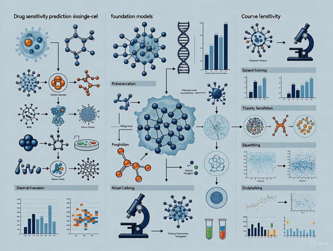
The standard workflow for drug sensitivity prediction involves multiple stages, from data preprocessing through model interpretation, as illustrated below:
Implementation Protocols
Protocol 1: Zero-shot drug sensitivity prediction using scFM embeddings
This protocol evaluates the intrinsic capability of scFMs to predict drug responses without task-specific fine-tuning [5] [7]:
- Input Preparation: Extract single-cell RNA-seq profiles from target cell populations (e.g., tumor biopsies) and format according to model-specific tokenization requirements [1]
- Embedding Generation: Process cellular profiles through pretrained scFM to obtain latent representations using zero-shot inference [5]
- Similarity Assessment: Compare query cell embeddings with reference profiles of annotated drug responses using cosine similarity metrics in the latent space [5]
- Response Prediction: Assign sensitivity scores based on proximity to known responsive or resistant cellular states in the embedding space [5] [7]
Protocol 2: Fine-tuned drug sensitivity classification
For enhanced performance on specific drug classes or cellular contexts, supervised fine-tuning is recommended [5] [4]:
- Data Curation: Compile labeled single-cell datasets with documented drug response outcomes (e.g., scRNA-seq of cancer cells pre- and post-treatment) [5]
- Model Adaptation: Append task-specific classification layers to the pretrained scFM and initialize with pretrained weights [4]
- Transfer Learning: Fine-tune the composite model on drug response labels using cross-entropy loss with balanced sampling to address class imbalance [5]
- Validation: Evaluate predictive performance on held-out test sets using multiple metrics including accuracy, AUC-ROC, and precision-recall characteristics [5]
Table 2: Performance Benchmarks of scFMs in Drug Sensitivity Prediction Tasks
| Model | Prediction Approach | Cancer Types Evaluated | Key Performance Metrics | Limitations |
|---|---|---|---|---|
| scGPT [5] [4] | Zero-shot & Fine-tuning | Multiple (Pan-cancer) | Strong overall performance across tasks | Computational intensity for fine-tuning |
| Geneformer [5] [4] | Representation transfer | Four cancer types | Effective gene-level prediction | Limited zero-shot capability |
| scFoundation [5] | Latent space projection | Seven cancer types | State-of-the-art in specific contexts | Inconsistent cross-dataset generalization |
| Baseline ML Models [5] [7] | Standard supervised learning | Benchmark comparisons | Efficient on targeted datasets | Poor transfer across biological contexts |
Essential Research Toolkit
Computational Frameworks and Reagents
Successful implementation of scFMs for drug sensitivity prediction requires specialized computational resources and frameworks:
Table 3: Essential Research Reagents and Computational Solutions for scFM Implementation
| Resource Category | Specific Tools | Functionality | Application Context |
|---|---|---|---|
| Integration Frameworks [2] [4] | BioLLM, DISCO, CZ CELLxGENE | Unified model access, standardized benchmarking | Cross-model comparison, reproducible analysis |
| Pretraining Corpora [1] [2] | Human Cell Atlas, CELLxGENE, GEO | Curated single-cell datasets for model training | Foundation model development, transfer learning |
| Specialized Architectures [2] | scGPT, Geneformer, scFoundation, EpiAgent | Domain-optimized model architectures | Task-specific applications, multimodal integration |
| Analysis Ecosystems [2] | scGNN+, BioLLM | Automated workflow optimization | Accessible implementation for non-specialists |
Critical Analytical Considerations
The effective application of scFMs for drug sensitivity prediction necessitates addressing several analytical challenges:
- Batch effect mitigation: Technical variation across datasets can confound biological signal, requiring careful preprocessing and batch-aware modeling [1] [2]
- Interpretability constraints: The black-box nature of transformer architectures complicates biological insight extraction, necessitating specialized interpretation tools [1] [6]
- Data quality requirements: High sparsity and noise in single-cell data impact model performance, emphasizing the need for rigorous quality control [1] [5]
- Computational resource demands: Training and fine-tuning large scFMs requires substantial GPU memory and processing capacity [1] [3]
The following diagram illustrates the key decision points in selecting an appropriate scFM strategy for drug sensitivity prediction:
Single-cell foundation models represent a powerful paradigm for predicting drug sensitivity at cellular resolution, offering unprecedented opportunities to understand heterogeneous treatment responses and identify novel therapeutic opportunities [5] [2]. The core principles of these models—including transformer architectures, self-supervised pretraining, and flexible adaptation mechanisms—enable them to capture complex biological relationships that traditional methods struggle to discern [1] [2].
While current implementations demonstrate promising capabilities, several challenges remain to be addressed, including improved interpretability, reduced computational requirements, and enhanced generalization across diverse biological contexts [1] [3] [7]. Future developments will likely focus on multimodal integration combining transcriptomic, epigenomic, and proteomic data [2], more biologically-informed architecture designs [5], and streamlined interfaces to broaden accessibility for biological researchers [3]. As these models continue to evolve, they hold substantial promise for accelerating therapeutic discovery and enabling more precise, personalized treatment strategies based on deep molecular profiling of individual cells [5] [2].
The advent of single-cell RNA sequencing (scRNA-seq) has fundamentally transformed biological research by enabling the investigation of cellular heterogeneity at unprecedented resolution. However, the data generated by these technologies—characterized by high dimensionality, extreme sparsity, and technical noise—presents significant analytical challenges [8] [1]. Inspired by breakthroughs in natural language processing (NLP), researchers have begun treating single-cell data as a distinct "language" where genes function as words and entire cellular transcriptomes as sentences [1]. This conceptual framework has paved the way for transformer-based foundation models, which leverage self-supervised learning on massive datasets to capture fundamental biological principles that can be adapted to diverse downstream tasks including drug sensitivity prediction, cell type annotation, and mechanistic inference [9] [8] [10].
This Application Note details how transformer architectures process single-cell data through a linguistic lens and provides detailed protocols for applying these models to predict drug sensitivity in cancer research. By framing biological data analysis within this paradigm, researchers can unlock deeper insights into cellular function and therapeutic response.
Foundation Models: Architectural Principles and Tokenization Strategies
Core Architecture Components
Single-cell foundation models (scFMs) predominantly utilize transformer architectures, which employ attention mechanisms to weight relationships between all genes within a cell simultaneously [1]. The self-attention mechanism enables these models to decide which genes in a cellular "sentence" are most informative for predicting the cell's identity or state, capturing complex regulatory relationships without predefined biological pathways [1].
Most scFMs employ either encoder-based architectures (like BERT) for classification and embedding tasks, or decoder-based architectures (like GPT) for generative modeling [1]. Hybrid designs are increasingly being explored to balance the strengths of both approaches for different biological applications. These models typically generate two types of output: gene embeddings that capture functional relationships between genes, and cell embeddings that represent the overall state or identity of a cell [8] [10].
Tokenization: From Biology to Computational Tokens
Tokenization converts raw gene expression data into structured inputs that transformers can process. Unlike words in natural language, genes lack inherent sequential ordering, requiring strategic approaches to sequence definition:
- Rank-based tokenization: Genes are ordered by expression level within each cell, creating a deterministic sequence from highest to lowest expressed genes [11] [1]. This approach provides robustness to technical variations.
- Value-based tokenization: Gene expression values are binned into discrete ranges, with each bin representing a different "word" in the vocabulary [1].
- Hybrid approaches: Some models incorporate both gene identifiers and their expression values as separate tokens, enabling the model to learn more complex relationships [8].
Additional special tokens are often incorporated to enrich biological context, including:
- Modality tokens indicating data types (e.g., scRNA-seq, spatial transcriptomics)
- Species tokens for cross-species learning
- Batch tokens to account for technical effects
- Cell-type tokens for supervised pretraining [11] [1]
Table 1: Common Tokenization Strategies in Single-Cell Foundation Models
| Strategy | Mechanism | Advantages | Representative Models |
|---|---|---|---|
| Rank-Based | Orders genes by expression level | Robust to batch effects, preserves gene relationships | Geneformer, Nicheformer |
| Value-Binning | Groups expression values into discrete bins | Captures absolute expression differences | scGPT |
| Hybrid | Combines gene ID and expression value tokens | Maximizes contextual information | scFoundation |
| Genomic Position | Orders genes by genomic coordinates | Leverages spatial genome organization | UCE |
Application Protocol: Drug Sensitivity Prediction with scGPT
Experimental Workflow and Design
The following protocol adapts the DeepCDR framework by integrating scGPT to predict drug sensitivity (IC50 values) from bulk RNA-seq of cancer cell lines, demonstrating how foundation models can enhance therapeutic prediction [10].
Table 2: Essential Research Reagents and Computational Resources
| Category | Item | Specification | Function/Purpose |
|---|---|---|---|
| Data Sources | Cancer Cell Line Encyclopedia (CCLE) | Bulk RNA-seq for 561 cancer cell lines | Provides gene expression inputs for model |
| Genomics of Drug Sensitivity in Cancer (GDSC) | IC50 values for drug-cell line pairs | Ground truth for model training/validation | |
| Computational Tools | scGPT | Pretrained foundation model (33M cells) | Generates cell embeddings from expression data |
| DeepCDR Framework | Hybrid graph convolutional network | Base architecture for drug response prediction | |
| Graph Neural Networks | Molecular structure processing | Encodes drug chemical information | |
| Hardware | GPU Resources | NVIDIA recommended (e.g., A100, V100) | Enables efficient model training/inference |
Step-by-Step Procedures
Data Preprocessing and Embedding Generation
Gene Expression Normalization
- Obtain bulk RNA-seq data from CCLE for cancer cell lines of interest.
- Normalize data using Counts Per Million (CPM) followed by log1p transformation to stabilize variance.
- Filter and align genes to match the expected input of scGPT (approximately 20,000 genes).
- Apply zero-padding for genes present in the scGPT reference list but absent from the expression dataset [10].
scGPT Embedding Generation
- Load the pretrained scGPT-human checkpoint (publicly available).
- Input preprocessed gene expression data into scGPT model.
- Extract the 512-dimensional cell embedding from the model output.
- Store embeddings for integration with drug representation data [10].
Drug Representation Processing
- Represent each drug as a molecular graph with:
- Feature matrix (75-dimensional) encoding atom attributes
- Adjacency list specifying bonds between atoms
- Degree list indicating neighbor counts for each atom
- Process drug graphs through a Graph Neural Network (GNN).
- Apply max pooling operation to summarize the most salient molecular features [10].
- Represent each drug as a molecular graph with:
Model Integration and Training
Feature Integration
- Concatenate the scGPT cell embedding (512-dimensional) with the drug representation from the GNN.
- Pass the concatenated representation through fully connected neural network layers.
Model Training and Validation
- Partition data into training (95%) and test (5%) sets.
- Use Mean Squared Error (MSE) loss between predicted and observed IC50 values.
- Implement leave-one-drug-out validation to assess generalizability to novel compounds.
- Evaluate performance using Pearson Correlation Coefficient (PCC) across cell lines, cancer types, and specific drugs [10].
Performance and Validation
The scGPT-enhanced DeepCDR framework demonstrates superior performance compared to both the original DeepCDR and scFoundation-integrated approaches:
- Prediction Accuracy: Achieves higher Pearson Correlation Coefficients (PCC) across cell line-based, cancer type-specific, and drug-specific evaluations [10].
- Generalization: Shows strong performance in leave-one-drug-out tests, indicating robust prediction capability for novel therapeutic compounds [10].
- Training Stability: Exhibits more consistent convergence and validation performance during training compared to alternative approaches [10].
Advanced Applications and Emerging Directions
Spatial Context Integration with Nicheformer
Recent advances incorporate spatial information through models like Nicheformer, trained on both dissociated single-cell and spatial transcriptomics data (SpatialCorpus-110M). This approach enables prediction of spatial context for dissociated cells, transferring rich microenvironmental information to standard scRNA-seq datasets [11]. Key applications include:
- Spatial composition prediction: Forecasting local cellular densities and neighborhood compositions
- Spatial label prediction: Annotating dissociated cells with spatial context (e.g., tissue layer, niche identity) [11]
Interpretability and Mechanistic Insight
Beyond prediction, transformer models enable mechanistic biological discovery through interpretability techniques:
- Attention mapping: Identifying genes with strongest influence on model predictions
- Feature importance: Using methods like SHAP to quantify contribution of individual genes to outcomes [9] [12]
- Rational biomarker discovery: Uncovering novel biomarkers by analyzing model decision patterns, such as the "Down Shift" white blood cell biomarker that complements existing inflammation markers [9]
Table 3: Benchmarking Single-Cell Foundation Models on Key Tasks
| Model | Pretraining Data | Key Applications | Drug Response Performance |
|---|---|---|---|
| scGPT | 33 million cells | Cell annotation, multi-omic integration, drug response | PCC: 0.85 (superior to baseline) |
| scFoundation | 50 million cells | Gene network inference, perturbation prediction | PCC: 0.82 (improved over DeepCDR) |
| Nicheformer | 110 million cells (incl. spatial) | Spatial context prediction, niche identification | N/A (specialized spatial tasks) |
| Geneformer | 30 million cells | Cell state transitions, network inference | N/A (limited drug response data) |
Troubleshooting and Technical Considerations
Common Implementation Challenges
Data Sparsity and Quality
- Challenge: High sparsity of scRNA-seq data impedes model performance.
- Solution: Implement gene embedding blocks to reduce sparsity effects, as demonstrated in scTransSort [13].
Computational Resource Limitations
- Challenge: Memory constraints during training with large datasets.
- Solution: Implement dataset slicing with consideration of potential bias introduction [10].
Batch Effect Integration
- Challenge: Technical variations between datasets affect model generalizability.
- Solution: Incorporate batch information as special tokens during training [1].
Model Selection Guidelines
When selecting a foundation model for drug sensitivity applications, consider:
- Dataset size: Simpler models may outperform foundation models with very small datasets [8]
- Task complexity: Complex tasks with limited training data benefit most from pretrained models [8]
- Interpretability needs: Models with built-in interpretability features (e.g., attention weights) support mechanistic insights [9]
- Computational resources: Larger models require significant GPU memory and training time [1]
Transformer-based foundation models represent a paradigm shift in single-cell data analysis, treating cellular transcriptomes as a language that can be decoded using advanced NLP-inspired architectures. The protocols outlined herein provide researchers with practical frameworks for applying these powerful models to drug sensitivity prediction, potentially accelerating therapeutic discovery and personalized treatment strategies. As these models continue to evolve—incorporating multimodal data, enhanced interpretability, and spatial context—they promise to unlock increasingly sophisticated insights into cellular biology and therapeutic response mechanisms.
The advent of single-cell RNA sequencing (scRNA-seq) has provided an unprecedented lens through which to view cellular heterogeneity, a critical factor in understanding differential drug responses. The computational analysis of this data, however, is fraught with challenges stemming from its high dimensionality, inherent sparsity, and technical noise [14]. Single-cell foundation models (scFMs), pre-trained on millions of cells, have emerged as powerful tools to overcome these hurdles. By learning universal patterns in transcriptomic data, these models provide a robust starting point for various downstream tasks, particularly in the realm of drug sensitivity prediction [8] [15]. Their ability to capture a deep understanding of gene-gene interactions and cellular states makes them uniquely suited for predicting how individual cells or populations will respond to therapeutic interventions. Among the plethora of scFMs, three key architectures—scBERT, scGPT, and Geneformer—exemplify different architectural philosophies and training strategies. Understanding their distinct mechanisms, strengths, and limitations is essential for researchers and drug development professionals aiming to harness their power for precision medicine. This article details the key architectural distinctions between these models and provides practical protocols for their application in predicting drug sensitivity.
The design of a foundation model—specifically, its choice of architecture, gene representation strategy, and pre-training objective—fundamentally shapes its capabilities and performance in downstream applications. The table below summarizes the core characteristics of scBERT, scGPT, and Geneformer.
Table 1: Key Architectural Characteristics of Featured Single-Cell Foundation Models
| Feature | scBERT | scGPT | Geneformer |
|---|---|---|---|
| Core Architecture | Encoder-only Transformer | Encoder-only Transformer (with generative pre-training) | Encoder-only Transformer |
| Primary Pre-training Task | Masked Gene Modeling (Classification) | Masked Gene Modeling (Regression & Generative) | Masked Gene Modeling (Contextual Rank Prediction) |
| Gene Representation | Value Binning (Categorization) | Value Binning & Value Projection | Gene Ranking (Ordering) |
| Model Parameters | ~40 million [8] | ~50 million [8] [16] | ~40 million [8] |
| Pre-training Scale | Millions of human cells [17] | 33 million human cells [17] [16] [18] | 30 million human cells [17] |
| Input Gene Count | 1,200 Highly Variable Genes (HVGs) [8] | 1,200 HVGs [8] | 2,048 ranked genes [8] |
Gene Representation Strategies
A critical differentiator among scFMs is how they convert continuous gene expression values into a format suitable for neural networks.
- Value Binning (scBERT, scGPT): This approach discretizes continuous expression values into a set of predefined "bins" or "buckets," effectively transforming regression into a classification problem [17] [14]. For example, scBERT might assign a gene with a certain expression level to a specific token ID representing "high expression." While this simplifies the modeling process, it can lead to a loss of fine-grained, quantitative information.
- Gene Ranking (Geneformer): Geneformer represents a cell by a sequence of gene names sorted in descending order of their expression value. This rank-based prioritization emphasizes the relative importance of genes within a cell and is inherently robust to batch effects and technical noise [17] [14]. Its pre-training task involves predicting the rank of masked genes within this contextual sequence.
- Value Projection (scGPT): In addition to binning, scGPT can also use a value projection strategy, where the continuous expression value is linearly projected into an embedding vector. This method preserves the full resolution of the expression data without discretization [17] [14].
Encoder-Centric Architectures
All three models—scBERT, scGPT, and Geneformer—are fundamentally based on the encoder-only Transformer architecture. Unlike decoder models that generate sequences autoregressively (like GPT for language), these models are designed to build rich, contextualized representations of their input data.
The encoder is composed of multiple layers of self-attention and feed-forward neural networks. The self-attention mechanism allows each gene in the input sequence to interact with every other gene, enabling the model to learn complex, non-linear gene-gene relationships that are crucial for understanding cellular state and, by extension, drug response [19]. The output is a dense embedding vector for each input gene, or a pooled embedding for the entire cell, which can then be used for classification, regression, or other downstream analyses.
scGPT's architecture is a notable variant, as it employs a generative pre-training objective within its encoder framework. It uses specialized attention masks during pre-training to predict the expression values of masked genes, allowing it to learn a generative understanding of cellular transcriptomes [16].
Diagram 1: Encoder Model Input-Output Workflow
Application Notes and Protocols for Drug Sensitivity Prediction
The following section provides detailed methodologies for applying scBERT, scGPT, and Geneformer to predict cancer drug response, a task critical for personalized medicine.
Protocol: Fine-tuning scGPT for Cell Line Drug Response Classification
This protocol outlines the steps to adapt the pre-trained scGPT model to predict the sensitivity of cancer cell lines to specific drugs.
Research Reagent Solutions:
- Pre-trained scGPT Model: The foundation model pre-trained on 33 million human cells, providing a general understanding of transcriptomics [18].
- Cancer Cell Line Dataset: A labeled dataset such as the Cancer Cell Line Encyclopedia (CCLE) or a proprietary dataset containing scRNA-seq profiles of cell lines and their measured IC50 values or binarized sensitivity labels for a drug of interest.
- Computational Environment: A GPU-equipped workstation (e.g., NVIDIA A100) with Python and the scGPT package installed via
pip install scgpt[18].
Step-by-Step Procedure:
- Data Preprocessing: Prepare your cell line expression matrix. Normalize the data using scGPT's builtin normalization functions and select the top 1,200 Highly Variable Genes (HVGs) to match the model's expected input dimension [8] [20].
- Model Initialization: Load the pre-trained scGPT "whole-human" model checkpoint using the provided
load_pretrainedfunction from the scGPT codebase [18]. - Classifier Head Attachment: Replace the model's pre-training head with a task-specific classification head. This is typically a fully connected (linear) layer that maps the final cell embedding to a probability distribution over the output classes (e.g., "sensitive" vs. "resistant").
- Fine-tuning: Train the model on your labeled cell line data. Freeze the initial layers of the transformer encoder if the dataset is small to prevent overfitting, and only fine-tune the later layers and the new classification head. Use a standard cross-entropy loss function and an Adam optimizer with a low learning rate (e.g., 1e-5).
- Evaluation: Assess the model's performance on a held-out test set of cell lines. Report standard metrics such as Area Under the ROC Curve (AUC), accuracy, and F1-score. The GRNFormer study, which built upon scGPT, demonstrated that such integration can lead to significant improvements in drug response prediction tasks [19].
Protocol: Zero-Shot Cell Embedding with Geneformer for Drug Sensitivity Analysis
This protocol describes how to use Geneformer in a zero-shot setting to generate cell embeddings that can be used as features for a separate drug response prediction model. This is particularly useful in discovery settings where labeled data is scarce or unavailable for fine-tuning [21].
Research Reagent Solutions:
- Pre-trained Geneformer Model: The model pre-trained on 30 million cells to understand gene context via rank-based modeling [8].
- In-house scRNA-seq Data: Unlabeled transcriptomic profiles from patient-derived cells or cell lines.
- External Drug Response Model: A machine learning classifier (e.g., Random Forest, Support Vector Machine) capable of predicting drug response from cell embeddings.
Step-by-Step Procedure:
- Input Preparation: For each cell in your dataset, create an input sequence for Geneformer by ranking the top 2,048 genes by expression level [8].
- Zero-Shot Inference: Pass each cell's gene rank sequence through the pre-trained Geneformer model without updating any of the model's parameters. Extract the cell's embedding from the model's output layer (e.g., the [CLS] token embedding or the mean of all gene embeddings).
- Feature Matrix Construction: Assemble the embeddings from all cells into a feature matrix, where each row is a cell and each column is a dimension of the embedding vector.
- Predictive Modeling: Use this feature matrix to train a separate, external drug response predictor if labels are available. The embeddings can also be used for unsupervised analysis, such as clustering, to identify cell subpopulations with potentially distinct drug sensitivity profiles. It is important to note that benchmarking studies have shown zero-shot performance can be variable, and may be outperformed by simpler methods like using Highly Variable Genes (HVGs) in some cases [21].
Protocol: Integrating Foundation Models into Multimodal Drug Response Pipelines
For the highest predictive accuracy, foundation models can be integrated as components within larger, multimodal deep learning frameworks that incorporate multiple data types.
Research Reagent Solutions:
- scFM Component: A single-cell foundation model (scGPT, Geneformer, or scBERT) to process transcriptomic data.
- Drug-Target Interaction (DTI) Model: A separately trained model, such as a Graph Neural Network (GNN), that generates embeddings from a drug's molecular structure and its protein targets [15].
- Multimodal Fusion Architecture: A neural network designed to combine embeddings from different modalities (e.g., transcriptomics and drug chemistry).
Step-by-Step Procedure:
- Process Each Modality:
- Cell Representation: Generate a cell embedding for a cell line or patient cell using one of the scFMs as described in Protocols 3.1 or 3.2.
- Drug Representation: Generate a drug embedding using the DTI model based on the drug's SMILES string or molecular graph.
- Feature Fusion: Concatenate the cell embedding and the drug embedding into a single, combined feature vector. More sophisticated fusion methods, such as cross-attention, can also be employed [19].
- Joint Prediction: Feed the fused feature vector into a final regression head (to predict a continuous value like IC50) or a classification head (to predict sensitive/resistant). The entire pipeline can be trained end-to-end.
- Validation: Rigorously validate the multimodal pipeline using leave-drug-out cross-validation to test its ability to generalize to novel therapeutics not seen during training. The DTLCDR model is an example of this approach, showing that integrating target information and single-cell language models significantly improves generalizability to unseen drugs [15].
Diagram 2: Multimodal Drug Response Prediction
The Scientist's Toolkit
Table 2: Essential Research Reagents and Computational Tools
| Item Name | Type | Function in Experiment | Example Source/Implementation |
|---|---|---|---|
| Pre-trained scGPT Checkpoint | Software/Model | Provides a foundational understanding of human transcriptomics for transfer learning. | scGPT GitHub repository "whole-human" model [18]. |
| Pre-trained Geneformer Checkpoint | Software/Model | Provides rank-based gene context understanding for zero-shot embedding generation. | Hugging Face Hub or original publication resources [8]. |
| Cancer Cell Line Encyclopedia (CCLE) | Dataset | Provides labeled scRNA-seq and drug sensitivity data for model training and validation. | Broad Institute DepMap Portal. |
| Harmony | Software Algorithm | Used for batch integration of scRNA-seq data from different sources to remove technical artifacts [21]. | R or Python package. |
| scVI | Software Algorithm | A generative model for scRNA-seq data used for normalization, dimensionality reduction, and batch correction [8] [21]. | Python package. |
| Flash-Attention Library | Software Library | Accelerates the self-attention computation in Transformer models, reducing training time and memory usage for scGPT. | Python package (pip install flash-attn) [18]. |
| Ascend/Atlas 800 Servers | Hardware | High-performance computing infrastructure with Ascend910 NPUs for large-scale model training. | Huawei (Used for training CellFM) [17]. |
Choosing the most appropriate single-cell foundation model for a drug sensitivity project depends on the specific task, data availability, and computational constraints. The following guide synthesizes insights from benchmarking studies and application notes to aid in this decision [8] [20] [21].
- Choose scGPT if: Your task requires high accuracy on a well-defined problem (e.g., cell line classification) and you have a labeled dataset for fine-tuning. Its generative pre-training and flexible input representation make it a powerful and versatile choice for supervised downstream tasks [16] [20].
- Choose Geneformer if: You are working in an exploratory setting with limited or no labels, and require robust, zero-shot cell embeddings for clustering or as features for a separate model. Its rank-based representation is highly effective at capturing biological signal amidst noise [17] [21].
- Consider a Simpler Baseline if: Computational resources are extremely limited or a benchmarking study on your specific data type shows that methods like Highly Variable Genes (HVG) selection combined with Harmony or scVI outperform foundation models in a zero-shot setting [21].
In conclusion, encoder-based models like scBERT, scGPT, and Geneformer have established a new paradigm for analyzing single-cell transcriptomic data in drug discovery. Their power lies in their pre-trained understanding of gene networks and cellular states. By following the detailed protocols provided—whether for fine-tuning scGPT, using Geneformer in zero-shot mode, or constructing a multimodal pipeline—researchers can effectively leverage these architectures to predict drug sensitivity with greater accuracy and biological insight, ultimately accelerating the development of personalized cancer therapies. Future advancements will likely involve tighter integration of multi-omics data and biological prior knowledge, as seen in models like GRNFormer, to further enhance predictive power and interpretability [19].
Single-cell foundation models (scFMs) represent a revolutionary approach in computational biology, leveraging large-scale deep learning models pretrained on vast single-cell datasets through self-supervised learning [1]. These models have emerged as powerful tools designed to overcome the inherent challenges of single-cell data analysis, including high dimensionality, technical noise, batch effects, and data sparsity [1] [5] [17]. Inspired by the success of transformer architectures in natural language processing, researchers have adapted these techniques to single-cell genomics, treating individual cells as "sentences" and genes or genomic features as "words" or "tokens" [1]. The fundamental premise of scFMs is that by exposing a model to millions of cells encompassing diverse tissues, species, and conditions, the model can learn universal biological principles that generalize effectively to new datasets and downstream tasks [1]. This pretraining paradigm is particularly valuable for drug sensitivity prediction, as it enables the model to capture fundamental aspects of cellular heterogeneity and regulatory mechanisms that underlie differential drug responses [22] [5]. The self-supervised nature of pretraining allows scFMs to learn from the rapidly expanding repositories of public single-cell data without requiring explicit labeling, making them exceptionally well-suited for extracting biologically meaningful representations that can be fine-tuned for specific predictive tasks in oncology and precision medicine [1] [22].
Core Architectures and Tokenization Strategies
Model Architecture Foundations
Most single-cell foundation models are built on transformer architectures, which utilize attention mechanisms to model complex dependencies between genes within individual cells [1] [17]. These architectures can be broadly categorized into encoder-based, decoder-based, and hybrid designs. Encoder-based models like scBERT employ bidirectional attention mechanisms that learn from all genes in a cell simultaneously, making them particularly effective for classification tasks and cell embedding [1]. In contrast, decoder-based models such as scGPT utilize a unidirectional masked self-attention mechanism that iteratively predicts masked genes conditioned on known genes, excelling in generative tasks [1]. Hybrid architectures that combine encoder and decoder components are also being explored to leverage the strengths of both approaches [1]. A recent innovation in this space is CellFM, which employs a modified RetNet framework with gated multi-head attention and Simple Gated Linear Units to achieve training parallelism and cost-effective inference while maintaining high performance [17]. The attention mechanisms in these architectures enable the model to learn which genes in a cell are most informative of cellular identity and state, capturing how genes covary across cells and their potential regulatory relationships [1].
Tokenization Approaches for Single-Cell Data
Tokenization converts raw gene expression data into discrete units that transformer models can process. Unlike words in natural language, genes lack inherent sequential ordering, presenting a unique challenge for applying transformer architectures to single-cell data [1] [5]. Three principal tokenization strategies have emerged, each with distinct advantages for capturing biological information:
Table: Tokenization Strategies in Single-Cell Foundation Models
| Strategy | Method Description | Representative Models | Advantages |
|---|---|---|---|
| Gene Ranking | Genes are ordered by expression levels within each cell to create a deterministic sequence | Geneformer, scGPT | Captures most highly expressed genes; provides natural ordering |
| Value Categorization | Continuous expression values are binned into discrete categories | scBERT, scGPT | Converts regression to classification; handles technical noise |
| Value Projection | Directly predicts raw gene expression values using linear projections | scFoundation, CellFM | Preserves full data resolution; maintains continuous nature of expression |
The gene ranking approach orders genes by expression magnitude, feeding the ordered list as a "sentence" to the model [1] [17]. Value categorization strategies discretize continuous expression values into bins or "buckets," transforming expression prediction into a classification problem [1] [17]. Value projection methods preserve the continuous nature of expression data by directly predicting raw values through linear projections [1] [17]. Beyond these core strategies, models often incorporate special tokens representing cell identity, modality, or batch information, and may enrich gene tokens with additional biological context such as gene ontology terms or chromosomal locations [1]. After tokenization, all tokens are converted to embedding vectors that combine gene identity and expression information, then processed by the transformer layers to produce latent embeddings for both individual genes and entire cells [1].
Data Curation and Pretraining Protocols
Data Sourcing and Curation
The development of robust scFMs requires massive, diverse, and high-quality single-cell datasets for pretraining. Researchers benefit from organized archives and databases that provide unified access to annotated single-cell data [1]. Platforms such as CZ CELLxGENE offer standardized access to over 100 million unique cells, while the Human Cell Atlas and other multiorgan atlases provide broad coverage of cell types and states [1]. Additional public repositories including the NCBI Gene Expression Omnibus (GEO), Sequence Read Archive (SRA), and EMBL-EBI Expression Atlas host thousands of individual single-cell studies [1]. The curation process involves meticulous data cleaning, quality control, and standardization. For example, CellFM aggregated 19,914 samples totaling approximately 100 million human cells from various public databases, followed by rigorous quality control filtering, gene name standardization according to HUGO Gene Nomenclature Committee guidelines, and conversion to a unified sparse matrix format [17]. This dataset included 46.3 million cells from normal donors and additional cells from diseased donors, with approximately 70 million cells having annotated cell types spanning diverse categories including T cells (19.2 million), mononuclear phagocytes (7.01 million), and neurons (6.29 million) [17]. Such comprehensive data curation ensures that the pretraining corpus captures a wide spectrum of biological variation essential for learning generalizable representations.
Self-Supervised Pretraining Objectives
Self-supervised learning objectives enable scFMs to learn meaningful biological representations without manual labeling. The most common pretraining tasks include:
Masked Gene Modeling: Inspired by masked language modeling in NLP, this approach randomly masks a subset of genes in each cell and trains the model to predict the masked values based on the remaining genes [1] [2]. This task forces the model to learn contextual relationships between genes and their coordinated expression patterns.
Next Gene Prediction: Utilizing decoder-based architectures, this method trains models to autoregressively predict the next gene in a sequence ordered by expression levels [1] [17]. This approach encourages the model to learn probabilistic dependencies between genes.
Contrastive Learning: This strategy trains models to recognize similar cellular states while distinguishing different ones, often by maximizing agreement between augmented views of the same cell while minimizing agreement with other cells [23]. Techniques such as random masking, Gaussian noise addition, or mutual nearest neighbor identification create positive and negative pairs for contrastive learning [23].
These self-supervised objectives allow the model to capture fundamental biological principles, including gene-gene interactions, regulatory relationships, and cellular state transitions, which form a foundational knowledge base transferable to various downstream tasks including drug sensitivity prediction [1] [22] [5].
Experimental Protocols for scFM Pretraining
Standardized Pretraining Workflow
The following protocol outlines a comprehensive procedure for pretraining single-cell foundation models, synthesizing best practices from established methods:
Step 1: Data Collection and Curation
- Source diverse single-cell datasets from public repositories (CELLxGENE, GEO, SRA, ENA, GSA, ImmPort) encompassing multiple tissues, conditions, and experimental platforms [1] [17].
- Implement rigorous quality control metrics: filter cells based on gene counts, mitochondrial percentage, and other quality measures; filter genes based on detection rates [1] [17].
- Standardize gene annotations according to HUGO Gene Nomenclature Committee (HGNC) guidelines to ensure consistent gene identity across datasets [17].
- Convert all data to a unified sparse matrix format for efficient storage and processing [17].
Step 2: Data Preprocessing and Normalization
- Apply appropriate normalization methods to address sequencing depth variations (e.g., library size normalization, log transformation) [1].
- Select highly variable genes to focus on biologically informative features and reduce computational complexity [5].
- For integration of multiple datasets, apply batch correction techniques that preserve biological variation while removing technical artifacts [5] [23].
Step 3: Tokenization Strategy Implementation
- Choose an appropriate tokenization strategy based on model architecture and research goals (gene ranking, value categorization, or value projection) [1] [17].
- Incorporate special tokens for cell identity, modality, or batch information when relevant [1].
- Enhance gene tokens with additional biological context such as gene ontology terms or chromosomal locations where available [1].
Step 4: Model Architecture Configuration
- Select transformer variant based on target applications: encoder architectures (e.g., BERT-like) for classification tasks, decoder architectures (e.g., GPT-like) for generation tasks, or hybrid designs for multifaceted applications [1].
- Configure model dimensions: embedding size, number of attention heads, number of layers, and feed-forward dimensions based on available computational resources and dataset size [1] [17].
- Implement efficient attention variants (e.g., RetNet, sparse attention) for large-scale training to reduce computational complexity [17].
Step 5: Self-Supervised Pretraining
- Implement masked gene modeling by randomly masking 15-30% of genes in each cell and training the model to reconstruct the masked values [1] [2].
- Utilize appropriate loss functions: mean squared error for continuous values, cross-entropy for categorized values, or contrastive losses for representation learning [1] [23].
- Train with large batch sizes and distributed training strategies across multiple GPUs or NPUs to handle the scale of millions of cells [17].
- Implement progressive training strategies: start with smaller subsets of data before scaling to full dataset [1].
Step 6: Model Validation and Evaluation
- Evaluate reconstruction accuracy on held-out validation datasets [1].
- Assess learned representations through zero-shot performance on downstream tasks such as cell type annotation, batch correction, or perturbation prediction [5] [23].
- Analyze biological relevance of embeddings by examining neighborhood relationships and functional enrichment [5].
Protocol for Fine-Tuning scFMs for Drug Sensitivity Prediction
Once a foundation model is pretrained, it can be adapted for drug sensitivity prediction using the following protocol:
Step 1: Task-Specific Data Preparation
- Collect single-cell RNA-seq data from cancer cells before drug treatment [22].
- Generate binary response labels (sensitive/resistant) based on post-treatment viability assays or established thresholds from databases like GDSC or CCLE [22].
- Address class imbalance using techniques such as SMOTE or oversampling, particularly important for drug response datasets where resistant cells may be underrepresented [22].
Step 2: Model Adaptation
- Extract cell embeddings from the pretrained foundation model [22] [5].
- Add task-specific prediction heads: multilayer perceptrons for direct classification or regression [22].
- Implement transfer learning approaches: fine-tune all parameters or use parameter-efficient methods like LoRA (Low-Rank Adaptation) [17].
- Incorporate attention mechanisms to identify genes critical for drug response prediction, enhancing both interpretability and performance [22].
Step 3: Model Training and Validation
- Split data into training, validation, and test sets, ensuring that cells from the same patient or experiment remain in the same split [22].
- Train with appropriate loss functions: binary cross-entropy for classification or mean squared error for continuous response values [22].
- Implement cross-validation strategies to assess model robustness [22] [5].
- Evaluate using multiple metrics: area under the ROC curve (AUC), average precision (AP), accuracy, and F1-score [22] [5].
Step 4: Interpretation and Biological Validation
- Analyze attention weights to identify genes and pathways important for drug response prediction [22] [5].
- Validate identified genes through differential expression analysis between sensitive and resistant cells [22].
- Visualize the transition from sensitive to resistant states using dimensionality reduction techniques like UMAP [22].
- Correlate model predictions with known biomarkers and pathways to assess biological plausibility [22] [5].
Performance Benchmarking and Evaluation
Quantitative Performance Comparison
Comprehensive benchmarking studies provide critical insights into the performance of scFMs across various biological tasks. The following table summarizes key performance metrics for established foundation models across tasks relevant to drug discovery:
Table: Performance Benchmarking of Single-Cell Foundation Models
| Model | Pretraining Scale | Cell Type Annotation Accuracy | Perturbation Prediction | Drug Response Prediction | Computational Efficiency |
|---|---|---|---|---|---|
| CellFM | 100M cells, 800M parameters | Superior cross-tissue annotation | High accuracy in gene function prediction | Not explicitly reported | Efficient RetNet architecture |
| scGPT | 33M cells | Robust zero-shot annotation | Strong perturbation modeling | Adaptable via fine-tuning | Moderate resource requirements |
| Geneformer | 30M cells | Context-aware embeddings | Good performance on perturbation tasks | Not explicitly reported | Rank-based efficiency |
| ATSDP-NET | (Fine-tuned approach) | Not primary focus | Not primary focus | Superior performance (Recall, ROC, AP) | Attention-based efficiency |
Recent benchmarks evaluating six scFMs against traditional methods reveal that no single model consistently outperforms others across all tasks, emphasizing the importance of task-specific model selection [5]. For drug sensitivity prediction, specialized approaches like ATSDP-NET, which combines transfer learning from bulk RNA-seq data with attention mechanisms, demonstrate superior performance with high correlation between predicted sensitivity gene scores and actual values (R = 0.888, p < 0.001) and resistance gene scores (R = 0.788, p < 0.001) [22]. In batch correction tasks, specialized frameworks like scVI and CLAIRE, along with fine-tuned scGPT, excel at removing technical variations while preserving biological signals [23]. For cell type annotation, generic self-supervised methods like VICReg and SimCLR sometimes outperform domain-specific approaches, particularly in cross-species and cross-tissue generalization [5] [23].
Evaluation Metrics and Biological Relevance
Rigorous evaluation of scFMs extends beyond traditional performance metrics to include biologically grounded assessment criteria:
Cell Ontology-Informed Metrics: Novel evaluation approaches like scGraph-OntoRWR measure the consistency of cell type relationships captured by scFMs with established biological knowledge from cell ontologies [5]. The Lowest Common Ancestor Distance (LCAD) metric assesses the severity of cell type misclassifications by measuring ontological proximity between predicted and true cell types [5].
Landscape Roughness Analysis: The Roughness Index (ROGI) quantifies the smoothness of cell property landscapes in the latent space, with smoother landscapes correlating with better generalization and easier training of task-specific models [5].
Knowledge-Based Evaluation: Beyond supervised metrics, evaluating the biological insights captured by models through gene set enrichment analysis, pathway activation patterns, and consistency with known biological hierarchies provides crucial validation of model utility [5].
Zero-Shot Transfer Capability: Assessing model performance on novel cell types, tissues, or species without additional fine-tuning measures the generalizability of learned representations [5] [2].
These multifaceted evaluation strategies ensure that scFMs capture not only statistical patterns but also biologically meaningful representations that can advance drug discovery and therapeutic development.
The Scientist's Toolkit: Essential Research Reagents
Table: Key Research Resources for scFM Development and Application
| Resource Category | Specific Tools/Platforms | Primary Function | Relevance to Drug Sensitivity Prediction |
|---|---|---|---|
| Data Repositories | CZ CELLxGENE, NCBI GEO, ENA, SPDB | Provide standardized access to single-cell datasets | Source of training data and benchmark datasets for model development |
| Computational Frameworks | MindSpore, PyTorch, TensorFlow | Enable model development and training | Support implementation of novel architectures and training strategies |
| Benchmarking Platforms | BioLLM, scSSL-Bench | Standardized evaluation of model performance | Enable comparative assessment of prediction accuracy and robustness |
| Specialized Models | scGPT, Geneformer, CellFM, ATSDP-NET | Pretrained models for specific applications | Provide foundation for transfer learning and fine-tuning approaches |
| Integration Methods | Harmony, scVI, CLAIRE | Batch correction and data integration | Ensure data quality and comparability across experimental conditions |
| Visualization Tools | UMAP, t-SNE, scGraph-OntoRWR | Interpretation and communication of results | Enable visualization of drug response transitions and cellular heterogeneity |
Pretraining strategies for single-cell foundation models have established a new paradigm for analyzing cellular heterogeneity and predicting drug sensitivity. By learning from millions of cells through self-supervised objectives, these models capture fundamental biological principles that enable accurate prediction of therapeutic responses at single-cell resolution [1] [22]. The integration of transformer architectures with biologically informed tokenization strategies creates representations that effectively capture the complex molecular interactions underlying drug sensitivity and resistance mechanisms [1] [22]. As evidenced by comprehensive benchmarking studies, scFMs demonstrate robust performance across diverse tasks but require careful selection based on specific application needs, dataset characteristics, and available computational resources [5] [23].
Future developments in scFMs for drug sensitivity prediction will likely focus on several key areas: enhanced multimodal integration combining transcriptomic, epigenomic, proteomic, and spatial data [2]; improved interpretability through biologically grounded attention mechanisms [22] [5]; federated learning approaches enabling model training across distributed datasets while preserving privacy [2]; and greater incorporation of biological prior knowledge through structured knowledge graphs [5] [2]. As these models continue to evolve, they will play an increasingly vital role in precision oncology and therapeutic development, ultimately enabling more accurate prediction of patient-specific treatment responses and uncovering novel mechanisms of drug resistance.
Single-cell RNA sequencing (scRNA-seq) has revolutionized biomedical research by enabling the investigation of gene expression at unprecedented cellular resolution. This technology provides detailed insight into cellular heterogeneity, revealing hidden cell diversity and complex biological processes that are obscured in bulk sequencing approaches [24]. However, the powerful insights gained from scRNA-seq come with significant computational challenges that must be addressed for meaningful biological interpretation, particularly in the context of drug sensitivity prediction.
The two primary technical challenges in scRNA-seq data analysis are high dimensionality and data sparsity [24]. scRNA-seq datasets typically contain measurements for thousands of genes across thousands to millions of cells, creating a high-dimensional space that is computationally intensive to process and analyze [25]. Furthermore, scRNA-seq data are characterized by exceptionally high sparsity, where a significant proportion of gene-cell combinations (often >90%) contain zero counts [26] [24]. These zeros represent a combination of biological factors (true absence of expression) and technical limitations (failure to detect expressed genes), commonly referred to as "dropout events" [27] [26].
For researchers developing drug sensitivity prediction models, these challenges are particularly acute. Accurate prediction of therapeutic responses requires distinguishing biologically relevant signals from technical artifacts, and the high sparsity can obscure critical gene expression patterns that determine drug sensitivity or resistance [28]. This application note provides detailed protocols and methodologies to overcome these challenges, with specific emphasis on applications in single-cell foundation models for drug sensitivity prediction.
Understanding scRNA-seq Data Characteristics
The sparsity and dimensionality of scRNA-seq data stem from both biological and technical factors. Biologically, individual cells naturally express only a subset of genes in the genome at any given time, creating legitimate zero counts. Technically, limitations in mRNA capture efficiency, reverse transcription, amplification, and sequencing depth contribute to additional zeros where expressed genes fail to be detected [27].
The term "dropout" specifically describes technical failures that cause highly expressed genes to be undetected [26]. However, usage has broadened in the literature to sometimes refer to all observed zeros. Recent evidence suggests that certain genes are consistently under-detected in scRNA-seq due to sequence-specific features. A comprehensive analysis of 53 paired bulk and scRNA-seq samples identified an enrichment of poly(T) motifs in the tails of frequently under-detected genes, which may form hairpin structures with poly(A) tails and impede mRNA capture during library preparation [26].
Quantitative Impact on Drug Response Prediction
The challenges of sparsity and dimensionality directly impact drug sensitivity prediction in several ways. Sparse data can obscure the expression patterns of critical drug response genes, particularly when these genes are expressed at low levels but have substantial biological effects. High dimensionality increases the risk of overfitting in predictive models, especially given the typically limited number of treated samples available for training [28].
Table 1: Characteristics of scRNA-seq Data That Impact Drug Sensitivity Prediction
| Characteristic | Typical Values | Impact on Drug Prediction |
|---|---|---|
| Cell-Gene Matrix Sparsity | >90% zeros [26] [24] | Obscures expression patterns of key drug response genes |
| Dimensionality | 20,000+ genes × 1,000-1,000,000+ cells [24] | Computational burden; high risk of overfitting |
| Dropout Rate Variability | Gene- and technology-dependent [26] | Introduces noise in feature selection for prediction models |
| Batch Effects | Multiple technical sources | Confounds drug response signals with technical variation |
For drug development professionals, these data characteristics necessitate robust preprocessing and analytical strategies. The ATSDP-NET model for single-cell drug response prediction addresses sparsity by combining transfer learning from bulk RNA-seq data with attention mechanisms to focus on informative genes, demonstrating how computational approaches can overcome these limitations [28].
Computational Strategies for Addressing Sparsity and Dimensionality
Dimensionality Reduction Techniques
Dimensionality reduction transforms high-dimensional gene expression data into lower-dimensional representations that retain essential biological information while reducing noise and computational requirements [24]. These techniques are fundamental for visualizing cellular heterogeneity and creating features for downstream predictive modeling.
Principal Component Analysis (PCA) is a linear dimensionality reduction method that identifies orthogonal directions of maximum variance in the data [25] [29]. PCA creates new uncorrelated variables called principal components (PCs), which are linear combinations of the original genes. The top 10-50 PCs that capture the majority of variance are typically retained for downstream analysis [25]. For scRNA-seq data, PCA is often applied after selecting highly variable genes to focus on biologically meaningful variation.
t-Distributed Stochastic Neighbor Embedding (t-SNE) is a non-linear graph-based technique that projects high-dimensional data into 2D or 3D space by defining a Gaussian probability distribution based on Euclidean distances between data points and recreating the distribution in low-dimensional space using Student t-distribution [25] [29]. t-SNE excels at revealing local structure and has demonstrated excellent performance in benchmarking studies, though it can be computationally intensive [29].
Uniform Manifold Approximation and Projection (UMAP) is another non-linear dimensionality reduction method that constructs a high-dimensional graph representation of the dataset and optimizes a low-dimensional graph to be structurally similar [25]. UMAP preserves more global structure than t-SNE while offering superior runtime performance, and has shown the highest stability in comparative evaluations [29].
Table 2: Comparison of Dimensionality Reduction Methods for scRNA-seq Data
| Method | Type | Strengths | Limitations | Best Use Cases |
|---|---|---|---|---|
| PCA [25] [29] | Linear | Computationally efficient; highly interpretable; preserves global structure | Limited to capturing linear relationships; less effective for visualization | Initial feature reduction; preprocessing for downstream algorithms |
| t-SNE [25] [29] | Non-linear | Excellent at revealing local structure and fine-grained clustering | Computationally expensive; loses global structure; sensitive to parameters | Visualization of cell subtypes and local neighborhoods |
| UMAP [25] [29] | Non-linear | Preserves both local and global structure; faster than t-SNE | Can produce overly connected clusters; parameter sensitivity | Visualization for trajectory inference; preprocessing for clustering |
| ZIFA [29] | Model-based | Explicitly models dropout events; handles zero-inflation | Limited to linear transformations; computationally intensive | Data with suspected high technical dropout rates |
| VAE/DCA [29] [24] | Deep learning | Captures complex non-linear patterns; integrates denoising | "Black box" nature; requires substantial computational resources | Large datasets; integration with deep learning pipelines |
Sparsity-Handling Approaches
Imputation methods aim to distinguish technical zeros from biological zeros and estimate values for the technical dropouts. Model-based imputation methods use probabilistic models to identify which observed zeros represent technical artifacts and impute expression values specifically for these cases [27]. For example, deep count autoencoder (DCA) denoises scRNA-seq data using deep learning with zero-inflated negative binomial loss functions, learning parameters of the negative binomial distribution to represent denoised reconstructions [29].
Data-smoothing approaches adjust all expression values based on similar cells, functioning as denoising methods rather than strict imputation [27]. These include diffusion-based methods like MAGIC, k-nearest neighbor approaches like knn-smooth, and network diffusion methods like netSmooth [27]. These methods can improve downstream analysis but risk introducing false signals if applied indiscriminately.
Data-reconstruction methods learn latent space representations through matrix factorization or autoencoders, implicitly generating less sparse reconstructions of the data [27]. Methods like ZINB-WaVE use zero-inflated negative binomial factor models, while variational autoencoders like scVI capture non-linear relationships while accounting for zero inflation [27].
Binary representations offer an alternative approach that embraces rather than corrects for sparsity. As datasets grow larger and sparser, several studies have demonstrated that binarized expression data (0 for zero counts, 1 for non-zero) can produce results comparable to count-based analyses for many applications, including dimensionality reduction, cell type identification, and differential expression [30]. Binary representations offer substantial computational efficiency, scaling up to ~50-fold more cells using the same resources [30].
Experimental Protocols for scRNA-seq Data Processing
Standardized Preprocessing Workflow
This protocol outlines a comprehensive workflow for processing raw scRNA-seq count data to address sparsity and dimensionality challenges, optimized for drug sensitivity prediction applications.
Materials and Reagents
- Raw scRNA-seq count matrix (genes × cells)
- Computational resources: Minimum 16GB RAM, multi-core processor
- Software environment: R (v4.0+) or Python (v3.8+)
- Key packages: Scanpy [25], Seurat [26], or equivalent scRNA-seq analysis toolkit
Procedure
Quality Control and Filtering
- Calculate quality metrics: total counts per cell, number of genes detected per cell, percentage of mitochondrial reads
- Filter out low-quality cells based on thresholds: typically <200 genes detected, >10-25% mitochondrial reads
- Remove genes expressed in fewer than 10 cells to reduce noise
Normalization
- Apply library size normalization to account for varying sequencing depths between cells
- Use methods tailored to scRNA-seq characteristics (e.g., SCTransform, or log1p normalization after size factor calculation)
- For UMI-based technologies, log1p transformation is often appropriate:
X_normalized = log(1 + X)
Feature Selection
- Identify highly variable genes using mean-variance relationships
- Select 2,000-5,000 most highly variable genes for downstream analysis
- This step dramatically reduces dimensionality while preserving biological signal
Dimensionality Reduction
- Apply PCA to normalized, highly variable genes
- Determine number of significant PCs using elbow method or statistical approaches
- Typically retain 10-50 PCs capturing majority of biological variance
- For visualization, apply non-linear methods (UMAP/t-SNE) to PC space
Batch Effect Correction (if multiple samples/datasets)
- Apply integration methods (Harmony, BBKNN, or Seurat's CCA) when combining datasets
- Particularly crucial for drug response studies combining multiple experiments
Troubleshooting Tips
- If cellular heterogeneity appears limited, adjust highly variable gene selection
- If batch effects persist, increase neighborhood size in integration methods
- For datasets with rare cell populations, use specialized methods (e.g., sctransform) to preserve rare cell signals
Protocol for Sparsity-Aware Drug Response Modeling
This protocol specifically addresses drug sensitivity prediction from sparse scRNA-seq data, incorporating strategies to handle sparsity without introducing significant bias.
Materials and Reagents
- Processed scRNA-seq data (post-QC and normalization)
- Drug response measurements (e.g., viability scores, IC50 values)
- Transfer learning resources: Pre-trained models on bulk RNA-seq (e.g., from GDSC/CCLE) [28] [31]
Procedure
Data Representation Selection
- For large, sparse datasets (>50,000 cells), consider binary representation (0/1) for computational efficiency [30]
- For smaller datasets with suspected high technical dropout, apply appropriate imputation (e.g., DCA, MAGIC)
- Validate representation choice by checking correlation between binary and count-based pseudobulk profiles [30]
Dimensionality Reduction for Feature Engineering
- Apply PCA to reduced gene set (highly variable or biologically relevant genes)
- For non-linear relationships, consider autoencoder-based reduction (e.g., scVI, DCA)
- For interpretable features, use methods that provide gene weights (PCA, BAE) [32]
Transfer Learning Implementation
Model Training and Validation
- Implement cross-validation strategies that preserve cell population structure
- Use appropriate metrics for drug response: ROC/AUC for classification, R² for continuous outcomes
- Apply regularization techniques to prevent overfitting to sparse features
Interpretation and Biological Validation
- Identify genes with highest attention weights as potential biomarkers
- Validate predictions using known drug response mechanisms
- Perform pathway enrichment on influential genes to contextualize predictions
Validation Methods
- Compare binary vs. count-based representations using silhouette scores in reduced dimension space [30]
- Validate imputation by measuring correlation with matched bulk RNA-seq where available [26]
- Assess transfer learning performance by comparing with and without pre-training
Advanced Methods and Emerging Approaches
Machine Learning and Deep Learning Approaches
Advanced machine learning methods are increasingly being applied to address scRNA-seq sparsity and dimensionality challenges, particularly for drug response prediction.
Transfer learning has emerged as a powerful strategy, leveraging large bulk RNA-seq drug response datasets (e.g., GDSC, CCLE) to improve generalization on smaller scRNA-seq datasets [28] [33]. The ATSDP-NET framework demonstrates how pre-training on bulk data followed by fine-tuning on single-cell data can significantly enhance prediction accuracy, with reported correlation values of R=0.888 for sensitivity gene scores and R=0.788 for resistance gene scores [28].
Attention mechanisms help models focus on the most informative genes and cells, effectively ignoring uninformative zeros in sparse data [28]. Multi-head attention allows models to capture different aspects of gene expression patterns relevant to drug response, improving both accuracy and interpretability.
Autoencoder architectures provide flexible dimensionality reduction while learning meaningful latent representations. Variational autoencoders (VAEs) like scVI explicitly model scRNA-seq noise characteristics, while denoising autoencoders (DAE) like DCA learn to reconstruct clean expression profiles from noisy inputs [29] [24]. The DrugS model employs autoencoders to reduce 20,000 protein-coding genes to just 30 features while retaining predictive power for drug response [31].
Boosting autoencoders (BAE) represent a recent innovation that combines componentwise boosting with neural networks to incorporate structural assumptions [32]. BAE identifies small gene sets that characterize latent dimensions, providing both dimensionality reduction and biological interpretability - particularly valuable for understanding drug response mechanisms.
Specialized Applications in Drug Sensitivity Prediction
Several specialized frameworks have been developed specifically for drug response prediction in single-cell data:
scDEAL utilizes bulk-to-single-cell transfer learning to predict drug responses at single-cell resolution, demonstrating the feasibility of leveraging existing large-scale drug screening data [28].
CaDRReS-SC employs latent space algorithms to model the relationship between drug action and cellular transcriptomic profiles, enabling prediction based on transcriptomic similarities [31].
ATSDP-NET combines transfer learning with multi-head attention mechanisms, showing superior performance across multiple metrics (recall, ROC, AP) in predicting sensitivity and resistance to compounds like I-BET-762 and cisplatin [28].
These approaches typically employ specialized preprocessing steps, such as TSNE clustering to exclude assay data with high variability within homogeneous clusters for the same drugs, ensuring more reliable training data [31].
The Scientist's Toolkit: Research Reagent Solutions
Table 3: Essential Computational Tools for Addressing scRNA-seq Sparsity and Dimensionality
| Tool/Resource | Function | Application Context | Key Advantages |
|---|---|---|---|
| Scanpy [25] | Comprehensive scRNA-seq analysis | End-to-end processing pipeline | Integration of multiple DR methods; seamless workflow |
| Seurat [26] | scRNA-seq analysis platform | Quality control through visualization | User-friendly; extensive documentation |
| SCANPY PCA [25] | Linear dimensionality reduction | Initial feature reduction | Computational efficiency; interpretability |
| UMAP [25] [29] | Non-linear visualization | 2D/3D visualization of cell states | Balance of local and global structure |
| DCA [29] | Denoising autoencoder | Handling technical noise | Explicit modeling of scRNA-seq noise characteristics |
| scVI [27] | Variational autoencoder | Large dataset integration | Probabilistic framework; batch correction |
| Harmony [30] | Dataset integration | Multi-sample batch correction | Preservation of biological variance |
| GDSC/CCLE [28] [31] | Drug response databases | Transfer learning pre-training | Large-scale drug response data |
| ZINB-WaVE [27] | Zero-inflated factor model | Handling excess zeros | Explicit zero-inflation modeling |
Workflow and Pathway Visualizations
Diagram 1: Comprehensive scRNA-seq Processing for Drug Response Prediction. This workflow integrates sparsity handling and dimensionality reduction strategies optimized for drug sensitivity prediction applications.
Diagram 2: Transfer Learning Framework for Drug Response Prediction. This architecture leverages bulk RNA-seq pre-training to overcome scRNA-seq data sparsity limitations while providing interpretable predictions through attention mechanisms.
From Data to Therapy: Implementing scFMs for Drug Response Prediction
Single-cell foundation models (scFMs) are large-scale deep learning models pretrained on vast single-cell omics datasets, capable of being adapted for various downstream tasks such as drug sensitivity prediction, cell type annotation, and batch integration [34] [1]. These models have revolutionized the interpretation of single-cell data by leveraging self-supervised learning on millions of cells to decipher the fundamental 'language' of cellular biology [34]. A critical preprocessing step that enables this paradigm is tokenization—the process of converting raw, unstructured gene expression data into structured, model-readable input sequences [34] [1]. Effective tokenization transforms the high-dimensional, sparse matrices characteristic of single-cell RNA sequencing (scRNA-seq) into meaningful token representations that preserve biological information while enabling computational efficiency [35]. For researchers focused on predicting drug sensitivity in heterogeneous cell populations, appropriate tokenization strategies are paramount for capturing the subtle transcriptional patterns that distinguish drug-sensitive from resistant subpopulations [36].
Core Tokenization Strategies and Architectures
Fundamental Approaches to Token Construction
Tokenization in single-cell analysis involves defining discrete input units (tokens) from gene expression data, analogous to words in a sentence for natural language processing [34]. In scFMs, individual cells are treated as documents or sentences, while genes or genomic features along with their expression values become the words or tokens [34] [1]. This conceptual framework allows models to learn the compositional rules of cellular identity and state. However, unlike words in natural language, genes lack inherent sequential ordering, presenting a fundamental challenge for transformer-based architectures that process sequential inputs [34] [5]. To address this limitation, several strategic approaches have been developed:
Expression-Based Ranking: Genes within each cell are ranked by expression levels, creating a deterministic sequence where the top highly expressed genes form the input "sentence" [34] [1]. This approach provides a consistent ordering scheme based on expression magnitude.
Expression Value Binning: Continuous expression values are partitioned into discrete bins, with each bin representing a different expression level category [34] [1]. The binned values then determine token positions or representations in the input sequence.
Normalized Count Representation: Some models forgo complex ranking strategies and directly use normalized count data with appropriate positional encoding schemes to represent gene order [34].
Each gene is typically represented as a token embedding that combines a gene identifier with its expression value in the given cell [34]. Special tokens may be prepended to enrich the input, including cell identity metadata, batch information, or modality indicators for multi-omics integration [34] [1]. Positional encoding schemes are then adapted to represent the relative order or rank of each gene in the cell, enabling the transformer architecture to process the non-sequential biological data effectively [34].
Comparative Analysis of Tokenization Methods
Table 1: Comparison of Primary Tokenization Strategies in scFMs
| Tokenization Approach | Mechanism | Advantages | Limitations | Representative Models |
|---|---|---|---|---|
| Expression-based ranking | Ranks genes by expression level per cell | Deterministic; prioritizes highly expressed genes | May overlook lowly expressed functional genes | Geneformer [34] |
| Expression value binning | Partitions continuous values into discrete bins | Captures expression intensity categories | Introduces arbitrary bin boundaries | scBERT [34] [35] |
| Normalized counts | Uses normalized expression values directly | Minimal preprocessing; preserves continuous nature | Requires careful normalization | scGPT [34] [35] |
| Full-gene tokenization | Processes all genes without selection | No biological information loss | Computationally intensive | scSFUT [35] |
Advanced Tokenization Frameworks for Drug Sensitivity Prediction
Specialized Tokenization for Clinical Applications
In the context of drug sensitivity prediction, tokenization strategies must capture not only cellular identity but also features predictive of therapeutic response. Advanced frameworks have emerged that address the specific challenges of clinical translation:
The Single-Cell Scale-Free and Unbiased Transformer (scSFUT) implements an innovative gene embedding approach using sequential tokenization and 1D-convolution to expand the attention receptive field of gene tokens [35]. This method processes high-dimensional scRNA-seq data at its original scale without requiring highly variable gene (HVG) selection, thereby avoiding the biological information loss that can obscure drug sensitivity signatures [35]. The model employs a mask-then-reconstruct self-supervised task that enables robust learning from high-sparsity data, crucial for identifying rare drug-resistant subpopulations [35].
For multi-omic integration in drug response prediction, models like scGPT incorporate modality-specific tokens that allow simultaneous processing of transcriptomic, epigenomic, and proteomic data from single cells [34] [1]. This approach enables the identification of coordinated molecular changes associated with drug resistance, such as simultaneous expression changes and chromatin accessibility alterations in resistance pathways [36].
Experimental Protocol: Implementing Tokenization for Drug Sensitivity Studies
Protocol 1: Expression-Based Ranking Tokenization for scFM Pretraining
Objective: Convert raw scRNA-seq count matrices into tokenized sequences suitable for foundation model pretraining, with emphasis on preserving features relevant to drug response prediction.
Materials:
- Raw single-cell RNA sequencing count matrix (cells × genes)
- High-performance computing environment with GPU acceleration
- Quality control metrics (minimum genes/cell, mitochondrial percentage)
- Normalization factors (library size, scaling factors)
- Gene identifier mapping file (Ensembl to common symbols)
Procedure:
- Quality Control and Filtering:
- Filter cells with fewer than 200 detected genes and genes expressed in fewer than 3 cells [35]
- Calculate quality metrics: total counts, mitochondrial percentage, ribosomal percentage
- Remove outliers based on quality metrics (typically >3 median absolute deviations from median)
Normalization:
- Apply library size normalization to counts per million (CPM) or log(CPM+1) transformation
- Alternatively, use scTransform or analytic Pearson residual methods for variance stabilization
Gene Selection:
Expression Ranking:
- For each cell, rank selected genes by normalized expression values in descending order
- Retain the top 2,048 genes (model-dependent) as the representative sequence for each cell [34]
Token Embedding Construction:
- Create token dictionary mapping each gene to an integer identifier
- Combine gene identifier with expression value (either continuous or binned) for embedding
- Add special tokens: [CLS] for cell-level representation, [BATCH] for batch correction, [DRUG] for perturbation studies
Positional Encoding:
- Apply sinusoidal or learned positional encodings based on gene rank in sequence
- For binning approaches, use bin index as positional reference
Validation:
- Assess tokenization quality by evaluating reconstruction loss in masked token prediction tasks
- Verify biological preservation through differential expression analysis in token embedding space
- For drug sensitivity applications, ensure separation of known sensitive and resistant populations in preliminary embeddings
Integrated Workflow for Drug Sensitivity Prediction
The complete workflow for applying tokenization strategies to drug sensitivity prediction encompasses multiple stages from data acquisition through model inference. The following diagram illustrates the integrated process:
Diagram 1: Integrated workflow for drug sensitivity prediction using tokenized single-cell data, highlighting the tokenization module as a critical component.
Research Reagent Solutions for scFM Implementation
Table 2: Essential Computational Tools for scFM Tokenization and Drug Sensitivity Prediction
| Tool/Category | Specific Examples | Function in Tokenization Pipeline | Application in Drug Studies |
|---|---|---|---|
| Data Repositories | CZ CELLxGENE, PanglaoDB, GEO/SRA | Provide pretraining corpora of annotated single-cell datasets | Source for drug perturbation atlases and resistant cell populations |
| Preprocessing Libraries | Scanpy, Seurat, Scater | Quality control, normalization, and highly variable gene selection | Batch effect correction across drug treatment conditions |
| Tokenization Frameworks | scGPT, Geneformer, scBERT | Implement gene ranking, binning, and embedding strategies | Incorporate drug response labels as special tokens |
| Model Architectures | Transformer Encoder (scBERT), Decoder (scGPT), Encoder-Decoder (scSFUT) | Process token sequences to generate latent representations | Predict IC50 values and resistance mechanisms from cell embeddings |
| Interpretation Tools | Attention visualization, scGraph-OntoRWR | Identify important genes and pathways through attention weights | Reveal molecular mechanisms of drug sensitivity and resistance |
Protocol for Domain-Specific Tokenization in Cancer Drug Response
Protocol 2: Multi-omic Tokenization for Cancer Drug Resistance Analysis
Objective: Implement modality-integrated tokenization for simultaneous analysis of transcriptomic and epigenomic features predictive of cancer drug resistance.
Rationale: Drug resistance in cancer often involves coordinated transcriptional and epigenetic adaptations [36]. Multi-omic tokenization enables modeling of these complex relationships.
Materials:
- Paired scRNA-seq and scATAC-seq data from cancer cell populations
- Cross-reference mapping between genomic regions and genes
- Multi-omic foundation model architecture (e.g., scGPT multi-omic extension)
- Drug sensitivity metrics (IC50, area under curve) for model supervision
Procedure:
- Modality-Specific Preprocessing:
- Process scRNA-seq data per Protocol 1
- Process scATAC-seq data: peak calling, count matrix generation, TF-IDF normalization
Cross-Modality Integration:
- Map scATAC-seq peaks to target genes using regulatory domain annotations
- Create paired feature set linking gene expression to regulatory activity
Multi-omic Tokenization:
- Create modality-specific tokens: [RNA] and [ATAC] prefixes
- For each cell, create interleaved token sequence alternating between:
- RNA tokens: (GeneID, ExpressionValue)
- ATAC tokens: (PeakID, AccessibilityValue)
- Add [DRUG_RESISTANCE] special token for fine-tuning on labeled data
Model Training and Fine-tuning:
- Pretrain on multi-omic corpus using masked token prediction
- Fine-tune on drug-treated samples with resistance labels
- Use attention weights to identify predictive features across modalities
Validation Metrics:
- Accuracy in predicting held-out drug response labels
- Enrichment of known resistance pathways in attention patterns
- Comparison to transcriptome-only models for predictive performance
Tokenization strategies form the critical bridge between raw biological data and powerful foundation models for drug sensitivity prediction. As scFMs continue to evolve, tokenization methods must advance to better capture the nuances of therapeutic response heterogeneity. Future directions include dynamic tokenization that adapts to specific biological contexts, integration of protein structure information for targeted therapies, and cross-species tokenization for translational drug development [35]. The standardized protocols and comparative frameworks presented here provide researchers with practical tools to implement these approaches in their drug sensitivity studies, ultimately contributing to more personalized and effective cancer therapeutics.
The advent of single-cell RNA sequencing (scRNA-seq) has revolutionized our understanding of cellular heterogeneity in health and disease, particularly in cancer biology. However, the high dimensionality, sparsity, and technical noise inherent to scRNA-seq data present significant challenges for computational analysis [5]. In parallel, the persistent challenge of drug resistance remains a major barrier to effective cancer therapy, with median response rates to FDA-approved cancer drugs remaining modest at approximately 41% [37].
Single-cell foundation models (scFMs) have emerged as powerful tools to address these challenges. Trained on millions of single-cell transcriptomes through self-supervised learning, these models learn fundamental biological principles that can be transferred to various downstream tasks [1]. Within this domain, three architectures—scGPT, UCE, and scFoundation—have demonstrated particular promise for drug response prediction at single-cell resolution, offering distinct approaches to a critical problem in precision oncology.
This application note provides a structured comparison of these three model architectures, detailing their operational mechanisms, performance characteristics, and practical implementation protocols for predicting drug sensitivity and resistance in single-cell data. By framing this analysis within the context of drug sensitivity prediction, we aim to equip researchers with the knowledge needed to select and implement appropriate models for their therapeutic investigations.
Comparative Analysis of Model Architectures
Performance Benchmarking in Drug Response Prediction
Comprehensive benchmarking studies provide critical insights into the relative strengths of scGPT, UCE, and scFoundation across different evaluation scenarios. The scDrugMap framework, which evaluated eight single-cell foundation models and two large language models on curated datasets encompassing 345,607 single cells, offers particularly valuable comparative data [37] [38].
Table 1: Model Performance in Pooled-Data Evaluation (Primary Data Collection)
| Model | Training Strategy | Mean F1 Score | Key Characteristics |
|---|---|---|---|
| scFoundation | Layer-freezing | 0.971 | Highest performance in pooled-data setting [37] |
| scFoundation | Fine-tuning (LoRA) | 0.947 | Maintains lead with parameter-efficient tuning [37] |
| scGPT | Fine-tuning (LoRA) | Competitive (exact value not reported) | Strong multi-omics capability [39] |
| UCE | Fine-tuning (LoRA) | Competitive (exact value not reported) | Effective in cross-data evaluation [37] |
| scBERT | Layer-freezing | 0.630 | Lowest performance in benchmark [37] |
Table 2: Model Performance in Cross-Data Evaluation Scenarios
| Model | Evaluation Scenario | Mean F1 Score | Key Advantages |
|---|---|---|---|
| UCE | Fine-tuning on tumor tissue | 0.774 | Highest performance after tissue-specific adaptation [37] |
| scGPT | Zero-shot learning | 0.858 | Superior generalization without target data fine-tuning [37] |
| scFoundation | Pooled-data evaluation | 0.971 | Excellent when data can be aggregated [37] |
The benchmarking results reveal that no single model dominates across all scenarios. scFoundation excels in pooled-data evaluations where models are trained and tested on aggregated data from multiple studies, achieving the highest mean F1 scores of 0.971 (layer-freezing) and 0.947 (fine-tuning) [37]. In contrast, for cross-data evaluation where models are tested on completely held-out studies, UCE achieves the highest performance (mean F1 score: 0.774) after fine-tuning on tumor tissue, while scGPT demonstrates superior capability in zero-shot learning settings (mean F1 score: 0.858) [37].
Architectural Characteristics and Implementation Considerations
Table 3: Architectural Specifications and Implementation Requirements
| Feature | scGPT | UCE | scFoundation |
|---|---|---|---|
| Core Architecture | Generative Pretrained Transformer (Decoder) [39] [40] | Not specified in detail | Transformer-based [37] |
| Parameters | 53 million [40] | Information missing | Information missing |
| Embedding Size | 512 [40] | Information missing | Information missing |
| Transformer Blocks | 12 [40] | Information missing | Information missing |
| Attention Heads | 8 per block [40] | Information missing | Information missing |
| Pretraining Data | CELLxGENE Census (33M+ cells) [39] [18] | Information missing | Information missing |
| Tokenization Strategy | Value binning [39] | Information missing | Value projection [14] |
| Key Strengths | Multi-omics integration, zero-shot learning [39] | Cross-data adaptation [37] | Pooled-data performance [37] |
The architectural differences between these models significantly impact their computational requirements and practical implementation. scGPT's 53 million parameters require substantial GPU memory for efficient training and inference [40]. In contrast, newer architectures like GeneMamba aim to address the quadratic complexity limitations of transformer-based models through state space models, offering linear computational complexity while maintaining competitive performance [14].
Experimental Protocols for Drug Response Prediction
scGPT Implementation for Zero-Shot Drug Response Prediction
Principle: scGPT leverages its generative pre-training on over 33 million cells to predict drug responses without task-specific fine-tuning, utilizing the model's inherent understanding of gene regulatory relationships [39] [18].
Protocol:
- Data Preprocessing:
- Input: Raw count matrix (Cells × Genes)
- Normalize using scGPT's builtin normalization (counts per 10,000 followed by log1p transformation)
- Filter genes and cells based on quality control metrics (mitochondrial percentage, minimum counts)
Model Loading:
- Download pretrained weights from the scGPT model zoo (prefer whole-human model for general applications)
- Initialize model with recommended hyperparameters (embedding size: 512, layers: 12, heads: 8)
- Set model to evaluation mode for inference
Zero-Shot Inference:
- Extract cell embeddings from the pretrained model
- Compute similarity metrics between query cells and reference drug response profiles
- Generate sensitivity/resistance predictions based on embedding neighborhoods
Validation:
- Compare predictions with ground truth labels where available
- Assess embedding quality using biological sanity checks (separation of known cell types)
scGPT Zero-shot Prediction Workflow
scFoundation Fine-Tuning with LoRA for Pooled Data Analysis
Principle: scFoundation achieves optimal performance in pooled-data scenarios through parameter-efficient fine-tuning using Low-Rank Adaptation (LoRA), which modifies model weights with minimal additional parameters [37].
Protocol:
- Data Pooling:
- Aggregate multiple single-cell datasets from different studies
- Apply robust batch correction while preserving biological variance
- Maintain consistent drug response labeling across studies
LoRA Configuration:
- Set rank parameter to balance adaptation capacity and overfitting risk
- Apply LoRA to attention mechanisms within transformer blocks
- Freeze base model parameters while training adapters
Training Procedure:
- Initialize with pretrained scFoundation weights
- Use Adam optimizer with learning rate of 0.0001
- Implement gradual unfreezing if full fine-tuning is required
- Monitor performance on held-out validation set
Evaluation:
- Assess F1 score, precision, and recall on test set
- Compare with baseline performance without fine-tuning
- Perform ablation studies on LoRA rank impact
scFoundation Fine-tuning with LoRA
UCE Cross-Data Evaluation Protocol
Principle: UCE demonstrates exceptional performance when trained on one dataset and evaluated on completely different studies, making it valuable for real-world scenarios where training data may not match application domains [37].
Protocol:
- Dataset Splitting:
- Partition data at study level rather than cell level
- Ensure no cells from test studies are seen during training
- Maintain balanced class distributions across splits
Domain Adaptation:
- Implement domain-invariant feature learning
- Utilize adversarial training or maximum mean discrepancy loss
- Preserve biologically relevant features while removing study-specific biases
Model Training:
- Fine-tune on source studies with strong regularization
- Employ early stopping based on validation performance
- Use learning rate scheduling for stable convergence
Cross-Study Validation:
- Evaluate on completely held-out studies
- Assess generalization across tissue types and cancer types
- Compare with study-specific trained models as baseline
Visualization of Model Comparison and Selection Framework
To facilitate appropriate model selection based on specific research constraints and objectives, we present a decision framework that incorporates key performance evidence from benchmarking studies.
Model Selection Decision Framework
The Scientist's Toolkit: Essential Research Reagents
Table 4: Key Research Reagents and Computational Resources
| Resource | Type | Function | Access |
|---|---|---|---|
| scDrugMap Framework | Software Platform | Integrated benchmarking of foundation models for drug response prediction [37] | https://scdrugmap.com/ [37] |
| CELLxGENE Census | Data Resource | Curated single-cell data for pretraining and validation [39] | https://cellxgene.cziscience.com/ [39] |
| scGPT Model Zoo | Pretrained Models | Collection of pretrained scGPT weights for different applications [18] | https://github.com/bowang-lab/scGPT [18] |
| GDSC/CCLE Databases | Drug Sensitivity Data | Bulk RNA-seq and drug response data for transfer learning [28] [41] | Public repositories |
| LoRA Implementation | Algorithm | Parameter-efficient fine-tuning for foundation models [37] | Standard in huggingface, scGPT |
| GeneMamba | Alternative Architecture | Efficient state space model for long sequences [14] | Emerging resource |
The practical application of scGPT, UCE, and scFoundation for drug sensitivity prediction requires careful consideration of research context, data availability, and performance requirements. scFoundation delivers exceptional performance when data from multiple studies can be aggregated, while UCE excels in cross-data scenarios requiring domain adaptation. scGPT offers compelling zero-shot capabilities valuable for exploratory analyses or when labeled training data is scarce.
Future developments in single-cell foundation models will likely address current limitations in interpretability, computational efficiency, and multimodal integration. Emerging architectures like GeneMamba demonstrate promising directions with more efficient state space models [14]. As these technologies mature, their integration into standardized drug discovery pipelines will accelerate the development of personalized cancer therapies and deepen our understanding of drug resistance mechanisms at single-cell resolution.
Researchers should consider establishing standardized benchmarking protocols specific to their experimental systems while maintaining flexibility to incorporate rapidly evolving model architectures. The field continues to progress toward more efficient, interpretable, and biologically grounded foundation models that will further enhance drug response prediction capabilities.
In the field of single-cell genomics, the advent of single-cell foundation models (scFMs) has revolutionized our ability to interrogate cellular heterogeneity and function at an unprecedented resolution. These models, trained on millions of single-cell transcriptomes, have emerged as powerful tools for diverse downstream biological analyses, including the critical challenge of predicting drug sensitivity in heterogeneous cell populations [8] [1]. The effectiveness of these models hinges on the strategic implementation of three core training workflows: pretraining, fine-tuning, and zero-shot learning. This document provides detailed application notes and experimental protocols for leveraging these workflows within the specific context of drug sensitivity prediction, offering researchers a structured framework for model development and application.
Core Concepts and Definitions
Single-Cell Foundation Models (scFMs)
Single-cell foundation models are large-scale deep learning models, typically based on transformer architectures, that are pretrained on vast and diverse collections of single-cell RNA sequencing (scRNA-seq) data. They learn universal representations of cellular states by treating individual cells as "sentences" and genes or genomic features as "words" or "tokens" [1]. The premise is that exposure to millions of cells across varied tissues and conditions enables the model to learn fundamental, generalizable principles of cellular biology.
The Triad of Training Workflows
- Pretraining: The initial, self-supervised phase where a model learns generalizable patterns and representations from a massive, unlabeled corpus of single-cell data. This phase is computationally intensive and establishes the model's foundational "knowledge" of cellular biology [1].
- Fine-Tuning: A subsequent supervised learning process that adapts a pretrained model to a specific task or domain—such as drug sensitivity prediction—by continuing training on a smaller, targeted dataset. This process updates the model's weights to specialize its performance [42] [43].
- Zero-Shot Learning: An approach where a pretrained model is applied to a novel task without any task-specific training. The model relies on its generalizable pretrained knowledge and semantic understanding to make predictions on classes or tasks it has never explicitly encountered during training [44].
Quantitative Comparison of Training Workflows
The choice between training workflows involves trade-offs between performance, resource requirements, and implementation speed. The following table summarizes these key considerations for scFM-based drug sensitivity prediction.
Table 1: Comparative analysis of training workflows for drug sensitivity prediction with scFMs.
| Workflow Characteristic | Pretraining | Fine-Tuning | Zero-Shot Learning |
|---|---|---|---|
| Primary Objective | Learn universal cellular representations from vast data [1] | Adapt a pretrained model to a specific predictive task [42] | Apply pretrained knowledge to novel tasks without further training [44] |
| Data Requirements | Massive, diverse scRNA-seq datasets (e.g., 30-50M+ cells) [8] [1] | Smaller, labeled drug response datasets | No additional training data required |
| Computational Cost | Very High (requires large GPU/TPU clusters) [43] | Moderate to High (depends on method) [42] | Very Low (inference only) |
| Implementation Time | Weeks to Months | Hours to Days [44] | Minutes [44] |
| Typical Performance on Specific Tasks | Not directly applicable for end tasks | High (can achieve state-of-the-art) [44] | Lower than fine-tuned models, but provides a strong baseline [44] |
| Best Suited For | Building new foundational models from scratch | High-stakes applications where maximum accuracy is critical | Rapid prototyping, tasks with limited or no labeled data, and benchmarking |
Application Notes for Drug Sensitivity Prediction
The Role of Pretraining
For most researchers, building a scFM from scratch is not necessary due to the availability of models like scGPT, Geneformer, and scFoundation [8] [1]. The primary application of pretraining in this context is to understand the source of a model's foundational knowledge. A model's effectiveness in downstream tasks like drug sensitivity prediction is directly influenced by the diversity and quality of its pretraining data. Models pretrained on corpora that include cancer cell states and perturbation data are likely to possess more relevant priors for drug response modeling [8].
When to Use Fine-Tuning vs. Zero-Shot Learning
The decision between fine-tuning and zero-shot learning is strategic and should be guided by project constraints and goals.
Use Fine-Tuning When:
- Maximum predictive accuracy is the paramount objective for your specific cell type and drug compound [44].
- You possess a sufficiently large, high-quality dataset of single-cell profiles with associated drug sensitivity measurements (e.g., IC50 values).
- Computational resources and time for additional training are available.
Use Zero-Shot Learning When:
Recent benchmarking studies reveal that no single scFM consistently outperforms all others across every task, including drug sensitivity prediction. Therefore, model selection should be tailored based on factors such as dataset size, task complexity, and the need for biological interpretability [8].
Experimental Protocols
Protocol 1: Zero-Shot Drug Sensitivity Analysis with a Pre-trained scFM
This protocol is designed for the rapid assessment of a pre-trained model's capability to infer drug sensitivity without further training.
I. Research Reagent Solutions
Table 2: Essential materials for zero-shot drug sensitivity analysis.
| Item | Function / Description |
|---|---|
| Pre-trained scFM (e.g., scGPT, Geneformer) | Provides the foundational model with embedded biological knowledge for inference [1]. |
| Target scRNA-seq Dataset | The query dataset containing single-cell transcriptomes from the biological system of interest (e.g., tumor biopsy). |
| Computational Environment (GPU recommended) | A machine with adequate memory and processing power to run large model inference. |
| Model-Specific Inference Scripts | Code provided by the model developers to generate cell embeddings or task-specific outputs. |
II. Step-by-Step Methodology
- Model and Data Acquisition: Download a pre-trained scFM and its associated tokenizer or data loader. Load your target scRNA-seq dataset, formatted as a gene expression matrix (cells x genes).
- Data Preprocessing and Tokenization: Normalize the target dataset using the model's predefined protocol (e.g., log(CP10K+1)). Convert the normalized expression matrix into a sequence of gene tokens. Most scFMs require ranking genes by expression level or binning expression values to create a deterministic input sequence [1].
- Embedding Generation: Pass the tokenized sequences through the pre-trained model in inference mode to extract latent cell embeddings. These embeddings are high-dimensional vectors that represent each cell's state as learned by the foundation model.
- Zero-Shot Prediction: Utilize the cell embeddings for downstream analysis. For drug sensitivity:
- Correlation Analysis: Correlate embedding dimensions with known markers of drug resistance/sensitivity.
- Clustering: Identify subpopulations of cells within the embeddings that may exhibit differential drug responses.
- Supervised Projection: Train a simple, shallow classifier (e.g., logistic regression) on a small subset of cells with known drug response to predict sensitivity on the remaining cells, using the fixed scFM embeddings as features.
The following diagram illustrates this workflow:
Protocol 2: Fine-Tuning an scFM for Drug Sensitivity Prediction
This protocol details the process of specializing a pre-trained scFM to predict drug sensitivity from single-cell data.
I. Research Reagent Solutions
Table 3: Essential materials for fine-tuning an scFM.
| Item | Function / Description |
|---|---|
| Pre-trained scFM | The base model to be adapted. |
| Labeled Drug Response Dataset | A dataset where single-cell profiles are paired with quantitative drug sensitivity labels (e.g., IC50, viability score). |
| Deep Learning Framework (e.g., PyTorch) | The software environment for implementing the training loop. |
| Parameter-Efficient Fine-Tuning (PEFT) Library (e.g., Hugging Face PEFT) | Provides implementations of methods like LoRA to reduce computational cost [43]. |
| GPU Cluster or High-Memory Cloud Instance | Hardware for handling the computational load of fine-tuning. |
II. Step-by-Step Methodology
- Task Formulation and Dataset Splitting: Define the prediction task as a regression (predicting IC50) or classification (sensitive vs. resistant) problem. Split your labeled dataset into training, validation, and test sets, ensuring that cells from the same patient or batch are not split across sets to prevent data leakage.
- Model Setup and PEFT Configuration: Load the pre-trained scFM. For parameter-efficient fine-tuning, configure a method like Low-Rank Adaptation (LoRA). LoRA freezes the original model weights and injects trainable low-rank matrices into the transformer layers, drastically reducing the number of parameters that need to be updated [43].
- Supervised Fine-Tuning Loop:
- For each batch of tokenized cell sequences from the training set, pass them through the model.
- The model's output (e.g., the embedding for a special
[CLS]token or the mean of all token embeddings) is fed into a task-specific prediction head (a small neural network). - The loss (e.g., Mean Squared Error for regression) between the prediction and the true drug sensitivity label is calculated.
- Backpropagation updates only the parameters of the LoRA adapters and the prediction head.
- Validation and Model Selection: Periodically evaluate the fine-tuned model on the held-out validation set. Save the model checkpoint that achieves the best performance on the validation metric.
- Final Evaluation: Report the final model's performance on the untouched test set to obtain an unbiased estimate of its predictive power for drug sensitivity.
The following diagram illustrates the fine-tuning protocol:
Integrated Analysis Workflow for Drug Development
A pragmatic approach for drug development pipelines is to sequentially employ zero-shot learning and fine-tuning. Researchers can first use a pre-trained scFM in zero-shot mode to gain initial insights and prioritize experiments. Subsequently, as validated drug response data is accumulated, fine-tuning can be employed to build a highly accurate, specialized predictive model. This hybrid strategy optimally balances speed and precision, accelerating the transition from genomic discovery to therapeutic candidate identification.
The accurate prediction of drug sensitivity is a cornerstone of precision oncology. While single-omics approaches have provided valuable insights, the intrinsic complexity and heterogeneity of cancer demand a more integrative strategy. The combination of gene expression profiles with mutation data and copy number variations (CNVs) offers a more comprehensive view of the tumor's functional state and genetic landscape, leading to significantly improved predictive models [45] [46]. This protocol details the methodologies for effectively integrating these multi-omics features, framed within the advanced capabilities of single-cell foundation models (scFMs), to enhance the prediction of cancer drug responses.
Background and Significance
Intratumor heterogeneity, driven by genetic, epigenetic, and functional differences among cancer cells, presents a major challenge for successful treatment. A significant source of this heterogeneity originates from DNA sequence variations and CNVs [47]. In fact, over 90% of solid tumors are aneuploid, and many exhibit chromosomal instability (CIN), leading to persistent karyotype changes [47]. Single-cell RNA sequencing (scRNA-seq) has revolutionized our ability to study this heterogeneity, and computational methods now allow for the inference of large-scale CNVs directly from scRNA-seq data, enabling a multi-faceted view of individual cells [48] [47].
The transition from single-gene level features to pathway-level analyses has emerged as a powerful approach. By computing the differences in multi-omics data within and outside biological pathways, models can capture more meaningful biological changes and improve interpretability [45]. Furthermore, the advent of scFMs, which are large-scale deep learning models pretrained on millions of single-cell transcriptomes, provides a robust foundation for analyzing cellular heterogeneity and complex regulatory networks [8] [1]. These models can be fine-tuned for specific downstream tasks, such as drug sensitivity prediction, by leveraging the rich biological knowledge encoded during pretraining.
Computational Methods and Protocols
Data Preprocessing and Multi-Omics Feature Extraction
A. Processing Single-Cell RNA-Sequencing Data
- Quality Control and Normalization: Begin with standard scRNA-seq preprocessing. Filter cells based on quality metrics (e.g., number of detected genes, mitochondrial read percentage). Normalize the gene expression counts using methods like Counts Per Million (CPM) followed by a log1p transformation (log(1+x)) to stabilize variance [10].
- Feature Selection: Select highly variable genes (HVGs) to reduce dimensionality and computational load for subsequent analysis. A common practice is to use the top 1,000-2,000 HVGs.
B. Inferring Copy Number Variations from scRNA-seq Data The following protocol is adapted from benchmarking studies and inferred CNV analysis [48] [47].
- Input: A normalized gene expression matrix (cells x genes) from the scRNA-seq data of the tumor sample.
- Reference Selection: Identify a set of diploid reference cells. For primary tissues, this can be normal cells from the same sample (e.g., cancer-associated fibroblasts or immune cells) identified via cell type annotation. For cancer cell lines, use an external dataset of healthy cells from a similar tissue type [48].
- CNV Inference: Apply a computational CNV caller. The choice of tool depends on the data type and required resolution (see Table 1).
- For expression-based inference: Use
InferCNVto calculate smoothed expression averages across genomic regions (e.g., chromosomes or chromosome arms) relative to the reference cells [47]. - For integrating allelic information: If single nucleotide polymorphism (SNP) data is available from the scRNA-seq reads, use
NumbatorCaSpER, which combine expression values with minor allele frequency information through a Hidden Markov Model (HMM) for more robust CNV calling [48].
- For expression-based inference: Use
- Output: A matrix of inferred CNV values per genomic region per cell.
C. Calling Single Nucleotide Variations from scRNA-seq Data
- Input: Aligned sequencing reads (BAM files) from scRNA-seq.
- Variant Calling: Use tools designed for scRNA-seq data (e.g.,
DENDRO) to call SNVs. Be aware of limitations: only SNVs in transcribed regions are covered, and allelic dropout (both biological and technical) is common, leading to missing data [46]. - Output: A binary genotype matrix (cells x SNVs) indicating the presence or absence of each called SNV.
Pathway-Level Feature Integration
This protocol is based on the PASO (Pathway and SMILES with Attention) model, which moves beyond single-gene features [45].
- Input: The three processed omics data matrices: Gene Expression, CNV, and Mutation.
- Pathway Database: Obtain gene sets for biological pathways (e.g., KEGG_MEDICUS from the MSigDB database).
- Calculate Pathway Difference Values:
- For Gene Expression and CNV Data: Use a non-parametric test like the Mann-Whitney U test to compute the difference in values for genes within a pathway versus genes outside the pathway.
- For Mutation Data: Apply the Chi-square-G test to assess the difference in mutation rates within and outside each pathway.
- Output: Three pathway-level feature matrices (one for each omics type), which serve as a more robust and interpretable input for the prediction model [45].
Integration with Single-Cell Foundation Models
This protocol describes enriching cell representations using a pretrained scFM, such as scGPT or scFoundation [8] [10].
- Model Selection: Download a pretrained scFM checkpoint (e.g., the scGPT-human model).
- Data Compatibility: Ensure your bulk or single-cell gene expression data is compatible with the model's expected input. This may require zero-padding for genes absent in your dataset but present in the model's predefined gene list.
- Generate Cell Embeddings: Pass the preprocessed (CPM normalized and log1p transformed) gene expression matrix through the scFM to extract a latent embedding for each cell. These embeddings, typically a 512-dimensional vector for scGPT, encapsulate the model's pretrained knowledge of cellular states [10].
- Feature Concatenation: Combine the scFM-derived cell embedding with the pathway-level CNV and mutation features (from section 3.2) into a unified feature vector representing each sample.
Drug Response Prediction Model Architecture
The following workflow integrates the prepared multi-omics features with drug information to predict sensitivity (e.g., IC50 value).
- Drug Representation: Represent each drug by its molecular structure using a Simplified Molecular-Input Line-Entry System (SMILES) string or a molecular graph. Process this representation using a Graph Neural Network (GNN) or multi-scale convolutional networks to extract drug features [45] [10].
- Multi-Omics Representation: Use the concatenated feature vector from section 3.3.
- Integration and Prediction: Employ an attention mechanism network to learn the complex interactions between the multi-omics features and the drug's chemical properties. Finally, feed the output into a Multilayer Perceptron (MLP) to generate the final drug response prediction (e.g., IC50) [45].
Figure 1: A workflow for multi-omics feature integration in drug sensitivity prediction, combining single-cell data, foundation models, and drug structural information.
Quantitative Data and Performance Comparison
Table 1: Benchmarking of scRNA-seq CNV Callers. Performance metrics are based on a benchmarking study evaluating six popular methods on 21 datasets with orthogonal ground truth (e.g., scWGS or WES) [48].
| Method | Input Data | Key Algorithm | Output Resolution | Key Performance Notes |
|---|---|---|---|---|
| InferCNV | Expression | Hidden Markov Model (HMM) | Per gene/segment | Widely used; good performance on plate-based data. |
| Numbat | Expression + Allelic Frequency | HMM | Per gene/segment | More robust in droplet-based data; requires SNP information. |
| CaSpER | Expression + Allelic Frequency | HMM | Per gene/segment | Robust for large datasets; requires SNP information. |
| SCEVAN | Expression | Segmentation | Per gene/segment | Good performance in identifying subclones. |
| copyKat | Expression | Segmentation | Per gene/segment | Effective for aneuploidy identification. |
| CONICSmat | Expression | Mixture Model | Per chromosome arm | Lower resolution; may be sufficient for large-scale CNVs. |
Table 2: Performance of Drug Sensitivity Prediction Models Integrating Multi-Omics Data.
| Model | Omics Features | Drug Representation | Key Innovation | Reported Performance (PCC) |
|---|---|---|---|---|
| PASO [45] | Pathway-level differences (Expr, CNV, Mut) | SMILES (Transformer) | Multi-scale CNN & pathway attention | Superior performance vs. other methods (exact PCC not stated) |
| DeepCDR [10] | Gene Expression (with scGPT) | Molecular Graph (GNN) | Integration of foundation model embeddings | scGPT-based DeepCDR outperformed original DeepCDR and scFoundation-based model |
| SAURON-RF [49] | Gene Expression | Not specified | Simultaneous regression & classification RF | Improved prediction for sensitive cell lines (exact PCC not stated) |
| CAISC [46] | SNV + CNV (integrated) | Not Applicable | Entropy-weighted integration of SNV/CNV | ARI = 0.97 (simulated data) vs 0.79 (SNV-only) & 0.74 (CNV-only) |
Table 3: Key Computational Tools and Datasets for Feature Integration in Drug Sensitivity Prediction.
| Resource Name | Type | Function | Access |
|---|---|---|---|
| InferCNV | Software/R Package | Infers CNVs from scRNA-seq data by comparing tumor and reference expression. | https://github.com/broadinstitute/inferCNV |
| Numbat | Software/R Package | Infers CNVs using HMM by integrating expression and allele frequency from scRNA-seq. | https://github.com/kharchenkolab/numbat |
| CAISC | Software/R Package | Integrates SNV and CNV data from scRNA-seq for subclonal identification. | https://github.com/lizamathews/CAISC |
| scGPT | Software/Python | A single-cell foundation model for generating enriched cell representations. | https://github.com/bowang-lab/scGPT |
| PASO | Software/Python | Deep learning model for drug response prediction using pathway-level multi-omics features. | https://github.com/queryang/PASO |
| GDSC | Database | Provides drug sensitivity (IC50) data for a wide range of cancer cell lines and drugs. | https://www.cancerrxgene.org/ |
| CCLE | Database | Provides multi-omics data (e.g., gene expression, mutation) for cancer cell lines. | https://sites.broadinstitute.org/ccle |
| CZ CELLxGENE | Database | A unified platform providing access to millions of single-cell datasets for pretraining. | https://cellxgene.cziscience.com/ |
The integration of gene expression with mutation and CNV data represents a paradigm shift in drug sensitivity prediction. By leveraging pathway-level analyses and the power of single-cell foundation models, researchers can build more accurate, robust, and interpretable models. The protocols and benchmarks provided here offer a practical roadmap for implementing these advanced computational strategies, ultimately contributing to the development of more effective personalized cancer therapies.
The accurate prediction of drug sensitivity represents a cornerstone of precision oncology. Current methodologies, predominantly based on bulk cell data, often fail to capture the profound heterogeneity within tumors, a key contributor to therapeutic failure and disease relapse [28] [50]. The advent of single-cell RNA sequencing (scRNA-seq) has unveiled unprecedented resolution into cellular diversity, creating an urgent need for computational models that can interpret drug responses at this granular level [22] [50]. This case study explores the integration of bulk and single-cell data through advanced deep learning frameworks to predict sensitivity to both targeted therapies and chemotherapeutics, situating these advancements within the broader pursuit of single-cell foundation models for drug response prediction.
Featured Computational Models and Performance
Recent innovations have produced several powerful models capable of predicting drug response by leveraging large-scale genomic and transcriptomic data. These models vary in their architecture, input data types, and interpretability features, as summarized in Table 1.
Table 1: Comparison of Featured Drug Sensitivity Prediction Models
| Model Name | Core Methodology | Input Data Types | Key Advantages | Reported Performance |
|---|---|---|---|---|
| ATSDP-NET [28] [22] | Transfer Learning + Multi-head Attention Network | Bulk & single-cell RNA-seq | Identifies key genes; superior accuracy on single-cell data | Recall, ROC, AP > benchmarks; Sensitivity gene score R=0.888 [28] |
| scDEAL [50] | Deep Transfer Learning (Domain-adaptive NN) | Bulk & single-cell RNA-seq | Infers signature genes for resistance; maintains single-cell heterogeneity | Avg. AUROC: 0.898; Avg. F1-score: 0.892 across 6 datasets [50] |
| DrugGene [51] | Visible Neural Network (VNN) + ANN | Gene mutation, expression, CNV; Drug fingerprints | High interpretability via biological pathways; integrates multiple data types | Outperforms existing methods (e.g., DrugCell) on same test set [51] |
| Histology Image Model [52] | Graph Neural Network (GNN) | H&E-stained Whole Slide Images (WSIs) | Uses routine histology; identifies spatial histological patterns | SCC > 0.5 for top 10 drugs [52] |
The ATSDP-NET model demonstrates the power of combining transfer learning with attention mechanisms. Pre-training on large bulk RNA-seq datasets like the Cancer Cell Line Encyclopedia (CCLE) and Genomics of Drug Sensitivity in Cancer (GDSC) allows the model to learn generalized gene-response relationships, which are then refined on single-cell data [28] [22]. The incorporated multi-head attention mechanism explicitly weights the importance of individual genes in the prediction, enabling both high accuracy and biological interpretability. The model has been validated on datasets involving human oral squamous cell carcinoma treated with Cisplatin and murine acute myeloid leukemia treated with I-BET-762, showing high correlation between predicted and actual sensitivity gene scores (R = 0.888, p < 0.001) [28].
In contrast, the scDEAL framework employs a Domain-adaptive Neural Network (DaNN) to harmonize the feature spaces of bulk and single-cell data [50]. It uses denoising autoencoders to extract robust low-dimensional features from both data types and minimizes the maximum mean discrepancy between them to facilitate effective knowledge transfer. A critical innovation in scDEAL is the integration of cell cluster labels into the loss function during training, which helps preserve the cellular heterogeneity inherent in scRNA-seq data that is often lost when integrating with bulk data [50].
The DrugGene model takes a different approach to interpretability by structuring its neural network according to known biological hierarchies [51]. Its Visible Neural Network (VNN) branch is built using Gene Ontology (GO) biological processes, allowing researchers to monitor the state of specific subsystems (e.g., signaling pathways) in response to genomic inputs. This pathway-level interpretation provides direct mechanistic insights into drug response.
Beyond transcriptomic data, emerging approaches demonstrate that drug sensitivity can also be predicted from routine histology images using graph neural networks. This method associates visual histological patterns in the tumor microenvironment with drug sensitivity profiles imputed from cell line data, providing a potentially more accessible predictive tool [52].
Experimental Protocol: Implementing the ATSDP-NET Framework
Data Acquisition and Preprocessing
- Bulk RNA-seq Data Source: Download bulk RNA-seq data and corresponding drug sensitivity measures (e.g., IC50 or AUC) from public databases such as GDSC [28] [31] or CCLE [51]. The drug response is often binarized into sensitive (1) and resistant (0) labels based on established thresholds [28] [22].
- Single-cell RNA-seq Data Source: Obtain scRNA-seq data (in count matrix format) from relevant studies or databases. The dataset should include pre-treatment transcriptomes and post-treatment viability assessments for each cell [28] [50].
- Data Harmonization: Normalize both bulk and single-cell datasets using a standardized method (e.g., log-transformation and scaling) to mitigate technical variations [31].
- Address Class Imbalance: Apply sampling strategies such as SMOTE or oversampling to ensure balanced classes in the training data [28] [22].
Model Training and Prediction
- Pre-training on Bulk Data: Initialize the model training using the large-scale bulk RNA-seq data to learn initial gene-response relationships. The model architecture should incorporate an attention mechanism [28].
- Transfer Learning to Single-Cell Data: Fine-tune the pre-trained model on the target single-cell RNA-seq dataset. This step adapts the bulk-derived knowledge to the single-cell context [28] [50].
- Prediction and Interpretation: Use the fine-tuned model to predict drug sensitivity (as a binary label or continuous probability) for individual cells. The attention weights can be extracted to identify genes most influential to the prediction [28] [22].
Validation and Analysis
- Performance Assessment: Evaluate model predictions against ground-truth labels using metrics such as Area Under the Receiver Operating Characteristic curve (AUROC), Average Precision (AP), and F1-score [50].
- Visualization: Project the results into a low-dimensional space using tools like Uniform Manifold Approximation and Projection (UMAP) to visualize the distribution of sensitive and resistant cells [28] [22].
- Biological Validation: Correlate the model-identified key genes with known markers of drug resistance or sensitivity through literature review or pathway enrichment analysis [28].
The following workflow diagram illustrates the core steps and data flow in a typical transfer learning approach for single-cell drug response prediction:
The Scientist's Toolkit: Research Reagent Solutions
Successful implementation of drug sensitivity prediction models relies on a suite of computational and data resources. Key reagents for this research are cataloged below.
Table 2: Essential Research Reagents and Resources for Drug Sensitivity Prediction
| Category | Resource Name | Description | Key Function in Research |
|---|---|---|---|
| Data Resources | Cancer Cell Line Encyclopedia (CCLE) [28] [51] | Comprehensive compilation of genomic data from human cancer cell lines. | Provides gene expression, mutation, and CNV data for model training. |
| Genomics of Drug Sensitivity in Cancer (GDSC) [28] [31] | Database linking drug sensitivity to genomic features in cell lines. | Source of drug response data (e.g., IC50) for supervised learning. | |
| Cancer Therapeutic Response Portal (CTRP) [52] [51] | Resource of drug sensitivity data from high-throughput screening. | Used for model training and validation. | |
| Computational Tools | Harmony [53] | Fast, scalable integration algorithm for single-cell data. | Corrects for technical batch effects across datasets before analysis. |
| UMAP [28] | Dimensionality reduction technique. | Visualizes high-dimensional data and model predictions (e.g., cell states). | |
| Scanpy / Seurat | Standard toolkits for single-cell RNA-seq analysis. | Used for primary data processing, normalization, and clustering. | |
| Experimental Materials | Human and Murine scRNA-seq Datasets | Pre-treatment transcriptomes with post-treatment viability labels. | Serves as the ground truth for model training and benchmarking [28] [50]. |
| Annotated Whole Slide Images (WSIs) | H&E-stained tissue sections from cancer cohorts (e.g., TCGA). | Enables histology-based prediction and spatial pattern analysis [52]. |
Signaling Pathways and Resistance Mechanisms
A primary advantage of interpretable models like ATSDP-NET and DrugGene is their ability to illuminate potential biological mechanisms underlying drug sensitivity and resistance. For instance, ATSDP-NET can highlight genes with high attention weights, pointing to specific pathways involved in the response to drugs like Cisplatin or I-BET-762 [28]. Similarly, the VNN in DrugGene tracks how input genomic alterations affect the state of entire biological subsystems, such as the PI3K-Akt, TNF, or NF-κB signaling pathways, which are frequently implicated in tumor survival and drug resistance [51] [31]. The following diagram conceptualizes how a genomic input is processed through a biologically structured model to yield a prediction and a mechanistic hypothesis.
Discussion and Future Perspectives
The integration of bulk and single-cell data through deep transfer learning represents a paradigm shift in drug sensitivity prediction. Models like ATSDP-NET and scDEAL effectively circumvent the data scarcity problem inherent in scRNA-seq studies by leveraging well-annotated bulk databases, while their attention mechanisms and interpretable architectures provide testable hypotheses about resistance mechanisms [28] [50]. The convergence of these models—handling diverse inputs from transcriptomics to histology—points toward a future of multi-modal foundation models in oncology.
These foundation models will likely be pre-trained on vast, multi-omic datasets, capable of being fine-tuned for specific tasks such as predicting response to a novel drug or identifying combination therapy targets in a patient-specific manner. The critical challenge remains the validation of these computational predictions in clinical settings. Future work must focus on bridging the gap between single-cell predictions and patient-level outcomes, potentially through the use of patient-derived models or the analysis of pseudo-bulk samples [28]. As these models evolve, they will increasingly inform clinical trial design and personalize therapeutic strategies, ultimately improving outcomes in cancer treatment.
Navigating Challenges: Practical Solutions for scFM Implementation
Data Quality and Batch Effect Mitigation Strategies
Single-cell RNA sequencing (scRNA-seq) has revolutionized biomedical science by enabling comprehensive exploration of cellular heterogeneity, individual cell characteristics, and cell lineage trajectories [54]. However, this technology introduces significant data quality challenges that profoundly impact downstream analyses, including drug sensitivity prediction. Technical artifacts arising from variations in tissue storage, dissociation processes, and sequencing library preparation often lead to inconsistent results and batch effects that can confound biological interpretation [54]. The inherent technical hurdles of scRNA-seq yield highly sparse data with high dimensionality, high sparsity, and low signal-to-noise ratios, further complicating result interpretation [8].
Batch effects represent technical variations irrelevant to study factors of interest that are introduced into high-throughput data due to variations in experimental conditions over time, use of different labs or machines, or employment of different analysis pipelines [55] [56]. Compared to traditional bulk RNA-seq technologies, scRNA-seq suffers from higher technical variations due to lower RNA input, higher dropout rates, and a higher proportion of zero counts, low-abundance transcripts, and cell-to-cell variations [55] [56]. These factors make batch effects more severe in single-cell data than in bulk data and have been shown to be predominant factors in large-scale and/or multi-batch scRNA-seq data analysis [55].
For drug sensitivity prediction models, particularly single-cell foundation models (scFMs), batch effects can introduce noise that dilutes biological signals, reduces statistical power, or even results in misleading, biased, or non-reproducible results [55] [56]. The profound negative impact of batch effects includes their role as a paramount factor contributing to irreproducibility, potentially resulting in retracted articles, invalidated research findings, and economic losses [55]. In clinical contexts, batch effects have led to incorrect classification outcomes for patients, some of whom received incorrect or unnecessary chemotherapy regimens [55] [56]. Therefore, implementing robust data quality control and batch effect mitigation strategies is essential for ensuring the reliability and reproducibility of drug sensitivity predictions derived from single-cell foundation models.
Quality Control Metrics and Procedures
Comprehensive Quality Control Framework
Implementing rigorous quality control (QC) is a crucial first step in single-cell RNA sequencing data analysis to ensure valid results before proceeding to batch effect correction and downstream drug sensitivity prediction [57]. The SCTK-QC pipeline provides a standardized framework for generating and visualizing QC metrics for scRNA-seq data, addressing five major types of QC analyses: (1) assessment of UMI and gene counts per cell, (2) empty droplet detection, (3) doublet/multiplet identification, (4) ambient RNA estimation, and (5) detection of biological artifacts [57]. This pipeline operates on three distinct data matrices: the "Droplet" matrix (containing all barcodes including empty droplets), the "Cell" matrix (empty droplets excluded), and the "FilteredCell" matrix (poor-quality cells further excluded) [57].
Table 1: Key Quality Control Metrics and Thresholds for scRNA-seq Data
| QC Metric Category | Specific Metrics | Interpretation Guidelines | Common Thresholds |
|---|---|---|---|
| Sequence Depth | Total UMIs per cell | Low counts indicate poor-quality cells; high counts may indicate multiplets | Dataset-dependent; typically exclude cells in extreme percentiles [54] |
| Gene Detection | Number of genes detected per cell | Low counts indicate poor-quality or dying cells | Dataset-dependent; typically exclude cells in extreme percentiles [54] |
| Cell Viability | Mitochondrial gene percentage | High percentages indicate stressed, apoptotic, or low-quality cells | 5-15%; varies by species, sample type, experimental conditions [54] |
| Doublet Indicators | Co-expression of marker genes from distinct cell types | May indicate doublets or transitional states | Requires manual inspection alongside automated tools [54] |
| Ambient RNA | Detection of cell-type-specific markers in inappropriate cell types | Suggests ambient RNA contamination | Use tools like SoupX or CellBender for removal [54] |
Transcriptional Quality Control Procedures
Ambient RNA contamination represents a significant challenge in scRNA-seq data quality, arising from transcripts leaked from damaged or apoptotic cells during single-cell isolation that become encapsulated in droplets along with other cells [54]. Additional transcription artifacts include barcode swapping due to incorrect binding between barcodes during sequencing [54]. These artifact transcripts complicate cell-type annotation by contaminating endogenous gene expression profiling and can lead to misinterpretation of biological differences. Several computational tools have been developed to address ambient RNA contamination: SoupX performs effectively without precise pre-annotation but requires manual input of marker genes and performs better with single-nucleus data compared to single-cell data, while CellBender is suited for cleaning up biological signals from noisy datasets and provides more accurate estimation of background noise [54].
Beyond ambient RNAs, specific gene classes should be considered for filtration, including ribosomal genes, immunoglobulin genes, human leukocyte antigen genes, and specific long non-coding RNAs, as they can induce unwanted batch effects in downstream clustering due to their overabundant expression and uncertain origination from various cell types [54]. Additionally, genes or cells associated with stress signatures induced by sample storage and dissociation should be carefully evaluated for removal, though caution is advised as stress-related gene expression can reflect genuine biological response and disease status [54].
Cellular Quality Control Procedures
Doublets or multiplets, where more than one cell is captured within a single droplet or microwell, represent significant technical artifacts that arise during scRNA-seq library preparation [54]. The multiplet rate is influenced by the scRNA-seq platform and the number of loaded cells; for example, 10x Genomics reports a 5.4% multiplet rate when 7,000 target cells are loaded, escalating to 7.6% with 10,000 target cells [54]. Several methods have been developed for doublet detection, each with distinct advantages: Scrublet demonstrates scalability for large datasets, doubletCells exhibits statistical stability across varying cell and gene numbers, and DoubletFinder outperforms other methods in accuracy and impact on downstream analyses like differential gene expression, clustering, and trajectory inference [54].
After removing transcript contamination and multiplets, additional filtering is recommended to exclude cells with excessively high or low gene/UMI counts, as high counts may indicate multiplet artifacts while low counts indicate potential low-quality cells [54]. Cells with mitochondrial percentage exceeding 5-15% should typically be excluded as low-quality cells, though these criteria must be adapted based on factors such as species, sample types, and experimental conditions [54]. For instance, human samples often exhibit higher mitochondrial percentages compared to mice, and highly metabolically active tissues like kidneys may display robust expression of mitochondrial genes [54].
The fundamental cause of batch effects can be partially attributed to the basic assumptions of data representation in omics data [55] [56]. In biomedical research, the measurement technologies aim to provide information about the concentration or abundance of an analyte in a sample, typically relying on the assumption that under any experimental conditions, there is a linear and fixed relationship between instrument readout and actual concentration [55] [56]. However, in practice, due to differences in diverse experimental factors, this relationship fluctuates, making instrument readouts inherently inconsistent across different batches and leading to inevitable batch effects [55] [56].
Table 2: Major Sources of Batch Effects in Single-Cell Studies
| Experimental Stage | Batch Effect Sources | Impact on Data Quality | Prevention Strategies |
|---|---|---|---|
| Study Design | Flawed or confounded design; minor treatment effect size | Systematic differences between batches; difficulty distinguishing biological signals from batch effects | Randomized sample collection; adequate sample size; balanced design [55] |
| Sample Preparation | Protocol procedures; reagent lots; storage conditions | Significant changes in mRNA, proteins, and metabolites | Standardize protocols; use same reagent lots; control storage conditions [55] [56] |
| Library Preparation | Personnel effects; equipment variations; timing differences | Technical variations introduced during processing | Use same personnel and equipment; process samples simultaneously when possible [58] |
| Sequencing | Different flow cells; sequencing batches; library concentrations | Batch-specific technical noise | Multiplex libraries across flow cells; balance samples across sequencing runs [58] |
| Data Analysis | Different processing pipelines; normalization methods | Inconsistent data processing artifacts | Standardize analysis pipelines; use consistent normalization approaches [55] |
Batch effects can emerge at every step of a high-throughput study, with some sources common across numerous omics types while others are exclusive to particular fields [55] [56]. During study design, flawed or confounded design represents a critical source of cross-study irreproducibility, occurring when samples are not collected randomly or are selected based on specific characteristics such as age, gender, or clinical outcome [55] [56]. The degree of treatment effect of interest also influences susceptibility to batch effects, as minor treatment effects make expression profiles more vulnerable to technical variations [55] [56]. In sample preparation and storage, variables in protocol procedures, reagent lots, and storage conditions can introduce technical variations that significantly impact high-throughput profiling results [55] [56].
Impact of Batch Effects on Drug Sensitivity Prediction
Batch effects have profound negative impacts on drug sensitivity prediction and other downstream analyses. In the most benign cases, batch effects increase variability and decrease power to detect real biological signals [55] [56]. When batch effects correlate with biological outcomes of interest, they can interfere with statistical analysis, leading to batch-correlated features being erroneously identified in differential expression analysis and prediction tasks [55] [56]. The challenges of batch effects are particularly magnified in longitudinal and multi-center studies, where technical variables may affect outcomes similarly to exposure variables, making it difficult or impossible to distinguish whether detected changes are driven by time/exposure or caused by batch effect artifacts [55] [56].
For drug sensitivity prediction using single-cell foundation models, batch effects can be especially problematic. Research has demonstrated that batch effect correction methods strongly impact differential gene expression analysis when sample size is large enough to contain sufficient information, thereby influencing downstream drug repositioning pipelines [59]. Studies comparing batch effect correction methods found that methods correcting for batch effects produced significantly better results than no correction for drugs with total sample sizes larger than 40 (drug and control samples combined) [59]. The external validity of gene signatures generated for drug repositioning depends critically on appropriate batch effect management, with the number of principal components included as covariates significantly influencing results [59].
Batch Effect Correction Methodologies
Computational Correction Strategies
Computational batch correction aims to remove technical variation from data, preventing this variation from confounding downstream analysis, including drug sensitivity prediction [58]. Multiple batch correction approaches have been developed, each with specific strengths and optimal application scenarios. Harmony is a valuable option for simple integration tasks involving distinct batch and biological structures, while for more complex integration tasks such as tissue or organ atlases, tools like single-cell Variational Inference (scVI) are more suitable [54]. BBKNN (Batch Balanced K Nearest Neighbours) has demonstrated excellent performance in handling scalable data concerning runtime and memory efficiency [54].
The performance of batch correction methods varies depending on scalability, complexity, and availability of cell annotations within the dataset [54]. For large-scale single-cell foundation models, the integration of multiple datasets requires careful consideration of batch effect correction strategies. Recent benchmarking studies of single-cell foundation models (scFMs) have evaluated their performance in batch integration alongside traditional methods, assessing their robustness and versatility across diverse applications [8]. While these foundation models show promise in handling heterogeneous datasets, simpler machine learning models sometimes demonstrate better efficiency in adapting to specific datasets, particularly under resource constraints [8].
Integration with Single-Cell Foundation Models
Single-cell foundation models (scFMs) represent a transformative approach to analyzing single-cell data, leveraging large-scale pretraining on diverse datasets to learn universal biological knowledge that can be adapted to various downstream tasks, including drug sensitivity prediction [8] [1]. These models typically use transformer architectures to incorporate diverse omics data and extract latent patterns at both cell and gene/feature levels, enabling sophisticated analysis of cellular heterogeneity and complex regulatory networks [1]. Most scFMs focus on single-cell RNA sequencing data but many can incorporate additional modalities such as single-cell ATAC sequencing, multiome sequencing, spatial transcriptomics, and single-cell proteomics [1].
A critical consideration for scFMs is their handling of batch effects and technical variations. While several models report robustness to batch-dependent technical biases without incorporating batch-specific tokens, others explicitly incorporate batch information as special tokens during the tokenization process [1]. The tokenization strategies vary across models, with some ranking genes by expression levels, others partitioning genes into bins by expression values, and some simply using normalized counts [1]. These different approaches influence how batch effects are managed within the model architecture itself.
SC Data Processing and Batch Correction Workflow
Experimental Protocols for Quality Control and Batch Correction
Comprehensive Quality Control Protocol
Protocol Title: Standardized Quality Control Pipeline for Single-Cell RNA Sequencing Data
Purpose: To systematically identify and remove low-quality cells, doublets, and ambient RNA contamination from single-cell RNA sequencing data prior to batch effect correction and downstream analysis for drug sensitivity prediction.
Materials:
- Raw single-cell count matrix (Droplet matrix)
- Computational resources with R/Python environment
- SingleCellTK package or equivalent QC tools
Procedure:
- Data Import and Initial Processing
- Import raw count data from preprocessing tools (CellRanger, BUStools, STARSolo, etc.)
- Combine multiple samples if applicable, retaining sample labels for batch identification
Empty Droplet Detection
- Apply barcodeRanks algorithm to rank all barcodes based on total UMI counts
- Compute knee and inflection points from log-log plot of rank against total counts
- Flag barcodes with total counts under knee or inflection points as empty droplets
- Alternatively, use EmptyDrops algorithm for more sensitive empty droplet detection
- Generate Cell matrix by excluding empty droplets [57]
QC Metric Calculation
- Calculate standard QC metrics: total UMIs per cell, number of genes detected per cell, mitochondrial percentage, ribosomal percentage
- Set appropriate thresholds for each metric based on experimental context and sample characteristics
- Identify cells with extreme values indicating poor quality or multiplets
Doublet Detection
- Apply multiple doublet detection algorithms (Scrublet, DoubletFinder, doubletCells)
- Compare results across methods to identify consensus doublet calls
- Manually inspect cells co-expressing markers of distinct cell types
- Determine whether co-expressing cells represent true transitional states or technical doublets
Ambient RNA Correction
- Estimate ambient RNA contamination using SoupX or CellBender
- For SoupX: provide marker genes for appropriate cell types through manual input
- For CellBender: leverage deep learning approach to estimate and remove background noise
- Generate corrected count matrix with reduced ambient RNA influence
Final Filtering and Data Export
- Apply comprehensive filtering to remove low-quality cells, doublets, and other artifacts
- Export FilteredCell matrix for downstream batch correction and analysis
- Generate QC report with visualization of key metrics across samples [57]
Troubleshooting Tips:
- If mitochondrial percentage thresholds are unclear, compare with similar studies using same species and tissue type
- If doublet detection algorithms show poor concordance, prioritize manual inspection of marker co-expression
- For heterogeneous samples, consider using sample-specific thresholds rather than global thresholds
Batch Effect Assessment and Correction Protocol
Protocol Title: Batch Effect Evaluation and Mitigation for Single-Cell Drug Sensitivity Prediction
Purpose: To identify, evaluate, and correct for batch effects in single-cell data to ensure reliable drug sensitivity predictions using foundation models.
Materials:
- FilteredCell matrix from quality control protocol
- Batch metadata (processing date, laboratory, reagent lots, etc.)
- Biological metadata (cell types, treatment conditions, etc.)
Procedure:
- Batch Effect Assessment
- Perform Principal Component Analysis (PCA) on normalized expression data
- Visualize sample distribution in PCA space, colored by batch and biological variables
- Identify whether samples cluster primarily by batch rather than biological factors
- Calculate batch effect metrics such as Average Silhouette Width by batch vs. biology
Method Selection for Batch Correction
- For simple batch structures with distinct biological groups: Select Harmony or Seurat Integration
- For complex integrations (tissue atlases, multiple conditions): Select scVI or BBKNN
- For large-scale data with runtime constraints: Prioritize BBKNN or Harmony
- When cell annotations are available: Utilize supervised or semi-supervised approaches
Batch Correction Implementation
- For Harmony: Run iterative clustering with dataset-specific clustering resolutions
- For Seurat Integration: Identify integration anchors across datasets then integrate
- For scVI: Train probabilistic model leveraging the deep generative framework
- For BBKNN: Construct batch-balanced k-nearest neighbor graph
Correction Quality Assessment
- Visualize corrected data in low-dimensional space (UMAP/t-SNE)
- Verify that biological groups are maintained while batch effects are reduced
- Calculate mixing metrics to ensure proper integration across batches
- Check that known biological structures are preserved post-correction
Integration with Foundation Models
- Prepare corrected data for foundation model training or fine-tuning
- For pretrained models: Ensure compatibility between correction method and model input requirements
- When using batch-aware foundation models: Provide batch information as special tokens
- Validate that batch-corrected data improves model performance on drug sensitivity prediction tasks
Validation Steps:
- Compare drug sensitivity predictions before and after batch correction
- Assess whether known drug response biomarkers become more significant after correction
- Verify that technical replicates show improved concordance after batch correction
- Ensure that biological meaningful variations are not removed during correction
Table 3: Essential Research Toolkit for Single-Cell Data Quality and Batch Effect Management
| Tool Category | Specific Tools/Resources | Primary Function | Application Context |
|---|---|---|---|
| Quality Control Tools | SoupX, CellBender, Scrublet, DoubletFinder | Remove ambient RNA, detect multiplets, filter low-quality cells | Preprocessing of raw scRNA-seq data prior to batch correction [54] [57] |
| Batch Correction Algorithms | Harmony, Seurat, scVI, BBKNN, MNN | Remove technical variations while preserving biological signals | Integration of multiple datasets/scenarios for robust analysis [54] [58] |
| Single-Cell Foundation Models | Geneformer, scGPT, scBERT, scFoundation | Learn universal representations from large-scale single-cell data | Drug sensitivity prediction, cell type annotation, batch integration [8] [1] |
| Benchmarking Frameworks | scGraph-OntoRWR, LCAD metrics | Evaluate biological relevance of model representations | Assessment of foundation model performance and biological accuracy [8] |
| Data Resources | CZ CELLxGENE, Human Cell Atlas, DepMap | Provide standardized single-cell datasets for training and validation | Pretraining foundation models, benchmarking method performance [1] |
Integrated Wet Lab and Computational Workflow
Effective management of data quality and batch effects is not merely a preprocessing step but a fundamental requirement for reliable drug sensitivity prediction using single-cell foundation models. The protocols and strategies outlined here provide a comprehensive framework for addressing these challenges throughout the experimental and computational pipeline. As single-cell technologies continue to evolve and foundation models become more sophisticated, the importance of rigorous quality control and appropriate batch effect correction will only increase.
Future directions in this field include the development of more integrated approaches that combine quality control and batch correction into unified frameworks, the creation of benchmark datasets specifically designed for evaluating batch effect correction in drug sensitivity contexts, and the incorporation of more sophisticated biological knowledge into correction algorithms. Additionally, as multi-modal single-cell data becomes more prevalent, methods capable of handling batch effects across different data types while preserving cross-modal relationships will be essential for advancing drug discovery and personalized medicine.
By implementing the quality control procedures, batch effect assessment strategies, and correction methodologies described in this document, researchers can significantly enhance the reliability and reproducibility of their drug sensitivity predictions, ultimately contributing to more effective therapeutic strategies and improved patient outcomes.
In the evolving field of drug sensitivity prediction using single-cell foundation models, the strategic choice between feature selection and feature transformation represents a fundamental methodological crossroad. Feature selection operates as a precision filter, identifying and retaining a subset of biologically meaningful variables—such as specific gene expressions or mutations—to enhance model interpretability and reduce overfitting [60]. In contrast, feature transformation creates new, condensed representations of all input features through mathematical projection or deep learning, often better capturing complex, non-linear relationships at the cost of direct biological interpretability [61].
This distinction is critical for single-cell drug sensitivity prediction, where the core challenge lies in distinguishing the transcriptional programs of cell type (stable identity) from cell state (transient, condition-responsive activity) [62]. The chosen approach directly impacts a model's ability to predict how a cell will respond to a compound. This document provides detailed application notes and experimental protocols to guide researchers in effectively applying these methods to build more accurate, interpretable, and robust predictive models.
Core Concepts and Quantitative Comparisons
Characterizing Feature Selection Approaches
Feature selection methods are categorized by their integration with the modeling process and their use of prior biological knowledge.
Table 1: Taxonomy and Characteristics of Feature Selection Methods
| Method Category | Core Principle | Advantages | Limitations | Exemplar Algorithms |
|---|---|---|---|---|
| Knowledge-Based Filter | Selects features based on prior biological knowledge or external databases (e.g., R-loop genes, cancer drivers). | High biological interpretability; independent of the predictor model. | Limited to known biology; may miss novel predictive features. | R-loop protein gene set [60]; Pathway-based selection. |
| Data-Driven Filter | Selects features based on intrinsic data properties (variance, correlation) without a predictor. | Computationally fast; model-agnostic. | May not select features optimal for the final prediction task. | Highly Variable Gene (HVG) selection; tF-sPBDS scoring [62]. |
| Wrapper | Evaluates feature subsets by their actual performance on the target predictive model (e.g., drug sensitivity). | Can find feature sets with high predictive power for the specific task. | Computationally intensive; high risk of overfitting. | Recursive Feature Elimination; LASSO for prognostic models [60]. |
| Embedded | Feature selection is built into the model training process itself. | Balances efficiency and performance; model-aware. | The selection process can be less transparent than filter methods. | LASSO regression [60]; Decision tree-based importance. |
Characterizing Feature Transformation Approaches
Feature transformation methods create new feature spaces, with a key divide between linear techniques and non-linear, deep learning-based approaches.
Table 2: Taxonomy and Characteristics of Feature Transformation Methods
| Method Category | Core Principle | Advantages | Limitations | Exemplar Algorithms |
|---|---|---|---|---|
| Linear Projection | Projects original features into a lower-dimensional space using linear combinations. | Simple, computationally efficient, and the components can sometimes be interpreted. | Assumes linear relationships, which is often a poor fit for complex biology. | Principal Component Analysis (PCA); Linear Discriminant Analysis. |
| Non-Linear Manifold Learning | Learns a low-dimensional, non-linear embedding that preserves the structure of the data. | Can capture complex, non-linear biological relationships. | Results can be sensitive to parameters; embeddings are often uninterpretable. | t-SNE; UMAP; PHATE. |
| Deep Learning / Foundation Model | Uses multi-layer neural networks to learn hierarchical, non-linear representations from data. | Extremely powerful for capturing intricate patterns; enables transfer learning. | "Black box" nature; requires large amounts of data and computational resources. | scSCC for clustering [63]; Omics consistency pre-training [61]. |
Strategic Selection: A Decision Workflow
The choice between selection and transformation is not mutually exclusive and should be guided by the study's primary objective. The following workflow diagram outlines a strategic decision-making process for method selection.
Application Notes for Drug Sensitivity Prediction
The Critical Role of Feature Selection in Deconvolving Cell Type and State
A pivotal challenge in multi-condition single-cell experiments (e.g., drug-treated vs. control) is that both cell type and cell state transcriptional programs are conflated. Using standard Highly Variable Gene (HVG) selection for clustering can group cells primarily by their treatment-induced state, obscuring true type-specific drug responses [62].
Solution: "Type-not-State" Feature Selection Wang et al. systematically evaluated feature selection strategies to disentangle these programs. Their findings advocate for a "type-not-state" strategy, which prioritizes genes that contribute to stable cell type identity while minimizing genes affected by the experimental condition (e.g., drug) [62].
- Quantitative Scoring for "Type-not-State": The protocol involves calculating separate scores for a gene's association with type (
tF,tPVE) and state (sPVE,sPBDS). Genes are then selected based on high type scores and low state scores (e.g.,tF-sPBDSstrategy) [62]. - Impact on Drug Sensitivity Analysis: When this selected gene set is used to construct the cell embedding space, it leads to:
- Cleaner Cell Type Clustering: Improved separation of cell types (higher Adjusted Rand Index).
- More Comparable Results: Increased consistency between different Differential State Analysis (DSA) methods like
muscatandmiloDEwhen identifying which cell types change in response to a drug [62].
This approach provides a more reliable foundation for downstream analysis of cell type-specific drug effects.
Feature Transformation and Foundation Models for Multi-Omics Integration
For complex tasks like predicting the sensitivity of a tumor cell line to a drug, no single data type provides a complete picture. Integration of gene expression, mutations, and drug structure is often necessary. Feature transformation, particularly via deep learning, is key to this integration.
Solution: Multi-Modal Foundation Model Pre-training One advanced method involves constructing separate graphs for drugs, genes, and cell lines. A foundation model is then pre-trained using omics consistency objectives, which force the model to learn a shared, meaningful embedding space for different data types [61].
- Pre-training Strategies:
- Predictive Consistency: The model is trained to predict one omics modality from another (e.g., gene expression from mutation profile).
- Contrastive Consistency: The model learns to pull embeddings of the same cell line from different modalities closer together, while pushing apart embeddings from different cell lines.
- Resulting Model: This generates a powerful, pre-trained feature transformer that encodes a tumor cell line into a rich, multi-omics representation. This representation can then be fine-tuned with a simple prediction head (e.g., a linear layer) to accurately predict drug sensitivity (e.g., IC50) [61]. This approach demonstrates how complex transformation can significantly boost predictive accuracy.
Experimental Protocols
Protocol 1: Knowledge-Guided Feature Selection for Prognostic Model Construction
This protocol details the construction of a drug sensitivity prognostic model using knowledge-based and statistical feature selection, as demonstrated in a study on lung adenocarcinoma [60].
I. Reagent Solutions
- R-loop Gene Set: A consolidated set of 1,551 R-loop binding protein genes from protein-protein interaction databases and R-loopBase [60].
- Clinical and Transcriptomic Datasets: Training set: TCGA LUAD (N=403). Validation sets: GEO datasets GSE14814 and GSE31210 [60].
- Software: R packages:
TCGAbiolinks,WGCNA,glmnet(for LASSO),survival,survminer.
II. Procedure
- Knowledge-Based Input Feature Compilation:
- Curate the initial R-loop gene set from literature and databases [60].
Data-Driven Module Detection via WGCNA:
- Perform quality control on the LUAD transcriptome data.
- Construct a weighted gene co-expression network using the
WGCNAR package. - Identify modules of highly co-expressed genes and correlate them with clinical traits (e.g., tumor grade, survival).
- Select the gene module with the strongest association to the clinical phenotype of interest for further analysis (e.g., 78 genes from the study) [60].
Regularized Regression for Feature Refinement:
- Subject the WGCNA-selected genes to Least Absolute Shrinkage and Selection Operator (LASSO) Cox regression.
- Use cross-validation to tune the penalty parameter
lambda, shrinking coefficients of less important genes to zero. - This step typically retains a smaller, more potent subset of genes (e.g., 14 genes) [60].
Multivariate Cox Regression for Final Model Building:
- Input the LASSO-selected features into a multivariate Cox proportional hazards model alongside key clinical variables (e.g., tumor grade).
- The final model will include only features that are independently predictive of prognosis (e.g., HEXIM1, GLI2, PLEC, and tumor grade) [60].
- Calculate a risk score for each patient using the formula:
Risk Score = Σ (Coefficient_i * Expression_i).
Validation:
- Divide patients into high- and low-risk groups based on the median risk score.
- Validate the model's prognostic power using Kaplan-Meier survival analysis and time-dependent ROC curves on the independent GEO validation sets [60].
The overall workflow for this protocol is illustrated below.
Protocol 2: Multi-Omics Consistency Pre-training for a Drug Sensitivity Predictor
This protocol describes a advanced feature transformation approach to create a foundation model for drug sensitivity prediction by learning a unified representation from multiple omics data types [61].
I. Reagent Solutions
- Omics Data: Gene expression and gene mutation profiles for tumor cell lines from CCLE or GDSC.
- Drug Data: Drug molecular structure (SMILES) and drug sensitivity measurements (e.g., IC50) from GDSC.
- Interaction Data: Protein-protein interaction network from the STRING database.
- Computing Environment: Python, deep learning frameworks (PyTorch/TensorFlow), graph neural network libraries.
II. Procedure
- Graph Construction:
- Drug Graph: Represent each drug as a graph where nodes are atoms and edges are chemical bonds.
- Gene Graph: Construct a gene/protein interaction network from STRING.
- Cell Line Feature Maps: Encode each tumor cell line as both a gene expression map and a gene mutation map [61].
Model Architecture Setup:
- Implement a tumor cell line encoder module (e.g., a Graph Neural Network or Transformer) to process the feature maps.
- Implement a drug encoder (e.g., a GNN) to process the drug graph.
Pre-training with Omics Consistency Objectives:
- Train the cell line encoder using a composite objective function that includes:
- Predictive Consistency: Minimize the loss of predicting gene expression from the mutation profile and vice-versa.
- Contrastive Consistency: Maximize the similarity (e.g., via InfoNCE loss) between embeddings of the same cell line generated from its expression and mutation maps [61].
- This step forces the model to learn a robust, integrated representation of the cell line.
- Train the cell line encoder using a composite objective function that includes:
Fine-tuning for Drug Sensitivity Prediction:
- After pre-training, connect the frozen or lightly fine-tuned cell line encoder and the drug encoder to a prediction head (e.g., a feed-forward network).
- Train the entire pipeline end-to-end on labeled drug-cell line pairs (e.g., IC50 values) from GDSC. The loss function is the mean squared error between predicted and actual sensitivity [61].
Model Evaluation:
- Evaluate the predictive performance on held-out test cell lines or drugs using metrics like Root Mean Square Error (RMSE) and Pearson correlation between predicted and true IC50 values.
The data flow and model architecture for this protocol are complex, as shown in the following diagram.
Table 3: Key Research Reagent Solutions for Feature Engineering in Drug Sensitivity
| Item Name | Function / Application | Exemplar Source / Identifier |
|---|---|---|
| R-loopBase | A knowledge database for obtaining R-loop binding protein genes for hypothesis-driven feature selection. | https://rloopbase.nju.edu.cn/ [60] |
| CCLE & GDSC Datasets | Primary sources of tumor cell line omics data (gene expression, mutation) and paired drug sensitivity measurements for model training and validation. | Cancer Cell Line Encyclopedia (CCLE); Genomics of Drug Sensitivity in Cancer (GDSC) [61] |
| STRING Database | Provides protein-protein interaction networks used to construct biological knowledge graphs for multi-omics models. | https://string-db.org/ [61] |
| tF-sPBDS Feature Scorer | A computational strategy for "type-not-state" feature selection in single-cell multi-condition experiments, improving differential analysis consistency. | [62] |
| scSCC Clustering Tool | A single-cell clustering algorithm using swapped contrastive learning, representing an advanced feature transformation for defining cell types. | [63] |
| Omics Consistency Pre-training Framework | A deep learning framework for pre-training a cell line encoder using predictive and contrastive losses on multi-omics data, creating powerful features for downstream prediction. | [61] |
The adoption of single-cell foundation models (scFMs) is transforming the landscape of drug sensitivity prediction and therapeutic development. These models, pretrained on massive single-cell transcriptomics datasets, offer the potential to predict cellular responses to genetic and chemical perturbations in silico, thereby accelerating drug discovery [1]. However, the burgeoning diversity of available scFMs presents a critical challenge: no single model consistently outperforms others across all tasks or datasets [5] [64]. Selecting the wrong model can lead to suboptimal performance, wasted computational resources, and unreliable biological predictions.
This Application Note establishes a standardized framework for selecting the optimal scFM based on specific task requirements, data resources, and biological contexts, with a particular emphasis on drug sensitivity prediction. By providing structured evaluation protocols, quantitative performance comparisons, and implementation guidelines, we empower researchers to make informed decisions that enhance the reliability and efficiency of their computational workflows in preclinical drug development.
Foundation Model Landscape and Core Selection Dimensions
Single-cell foundation models are typically built on transformer architectures and trained on millions of single-cell transcriptomes using self-supervised objectives [1]. They learn a universal representation of genes and cells, which can be adapted to various downstream tasks. The table below summarizes key models and their primary characteristics.
Table 1: Key Characteristics of Prominent Single-Cell Foundation Models
| Model | Architecture Type | Pretraining Scale | Notable Strengths | Reported Limitations |
|---|---|---|---|---|
| scGPT [64] | Decoder (GPT-like) | Large-scale | Robust performance across diverse tasks; effective batch correction; strong zero-shot embeddings. | - |
| Geneformer [5] [65] | Transformer | 30M+ cells (e.g., 30M-12L model) | Strong gene-level task performance; effective for in silico perturbation prediction. | Lower performance on some batch integration tasks. |
| scFoundation [5] [64] | Transformer | Large-scale | Strong performance on gene-level tasks. | Higher computational resource requirements. |
| scBERT [64] | Encoder (BERT-like) | Smaller scale | Early pioneer for cell type annotation. | Lagged performance likely due to smaller size and limited training data. |
A Multi-Dimensional Framework for Model Selection
Choosing the right scFM requires a balanced consideration of multiple interdependent dimensions. The following diagram illustrates the core decision-making workflow.
The framework prioritizes four core dimensions:
- Task Complexity and Type: Model performance varies significantly across tasks [5]. Cell-level tasks (e.g., batch integration, cell type annotation) often favor models like scGPT, while gene-level tasks (e.g., drug sensitivity prediction, perturbation modeling) may be better suited for Geneformer or scFoundation.
- Data Resources: The volume and quality of available data for fine-tuning are critical. For large, diverse datasets, complex scFMs excel. However, under resource constraints or with smaller datasets, simpler machine learning models can sometimes adapt more efficiently and outperform scFMs [5].
- Computational Resources: Model size, inference time, and memory footprint are practical constraints. scGPT and Geneformer are noted for superior computational efficiency compared to other large models [64].
- Biological Interpretability: For applications like target identification, the model's ability to provide biologically plausible insights is crucial. Emerging metrics like scGraph-OntoRWR, which evaluates the consistency of model-derived cell relationships with established biological knowledge, are vital for this dimension [5].
Quantitative Performance Benchmarks
Systematic benchmarking provides the empirical foundation for model selection. The following tables summarize key performance metrics from recent large-scale evaluations, focusing on tasks relevant to drug discovery.
Table 2: Benchmarking scFMs on Core Analysis Tasks (Performance Rankings)
| Model | Cell Type Annotation (Accuracy) | Batch Integration (ASW Score) | Perturbation Prediction | Zero-Shot Embedding Quality |
|---|---|---|---|---|
| scGPT | Leading [64] | Leading (Superior batch mixing & biological preservation) [64] | Moderate (Challenges in zero-shot) [66] | High (Consistently superior ASW) [64] |
| Geneformer | Moderate | Moderate (Distinguishes certain types) [64] | Leading (Used in closed-loop frameworks) [65] | Moderate |
| scFoundation | Moderate | Moderate | Strong in gene-level tasks [5] [64] | Moderate |
| scBERT | Lower | Lower (Poor performance) [64] | Not Highlighted | Low (Declines with longer input) [64] |
| Standard Baseline (e.g., PCA) | - | Lower than scGPT [64] | Can be competitive with scFMs [66] | - |
Table 3: Performance in Clinically Relevant Tasks (e.g., Drug Sensitivity Prediction)
| Model / Approach | Task Specificity | Key Performance Metric | Result / Insight |
|---|---|---|---|
| Fine-tuned scFMs (General) | Drug Sensitivity Prediction across 7 cancer types & 4 drugs [5] | Holistic Ranking | scFMs are robust and versatile, but no single model is universally best. Selection is context-dependent. |
| Closed-loop Geneformer [65] | In silico Perturbation (ISP) for target discovery | Positive Predictive Value (PPV) | Increased PPV from 3% (open-loop) to 9% by incorporating experimental data. |
| Open-loop Geneformer [65] | In silico Perturbation (ISP) for T-cell activation | Negative Predictive Value (NPV) | Showed high NPV (98%), outperforming differential expression (DE). |
| Zero-shot scFM Embeddings [66] | Perturbation Effect Prediction | Comparison to Baseline | Offer limited improvement over simple baseline models, especially under distribution shift. |
Experimental Protocols for Model Evaluation
To ensure reproducible and reliable model selection, researchers should implement standardized evaluation protocols. The following workflow details a comprehensive strategy for assessing scFM performance, with a focus on drug sensitivity prediction.
Comprehensive Model Evaluation Workflow
Protocol 1: Evaluating Perturbation Effect Prediction for Drug Sensitivity
This protocol assesses a model's ability to predict transcriptional responses to chemical or genetic perturbations, a core task in MoA (Mechanism of Action) studies and target validation.
- Objective: Systematically evaluate the accuracy of scFMs in predicting gene expression changes following a perturbation relevant to a disease model (e.g., gene knockout, drug treatment).
- Input Data Requirements:
- A held-out perturbation dataset (e.g., from Perturb-seq) not seen during the model's pretraining.
- A negative control dataset (unperturbed cells) from the same biological context.
- Procedure:
- Step 1: For the model in a zero-shot or fine-tuned setting, generate latent embeddings for both perturbed and unperturbed control cells.
- Step 2: Train a simple classifier (e.g., logistic regression) on these embeddings to distinguish between the two conditions.
- Step 3: Quantify model performance using metrics such as AUROC (Area Under the Receiver Operating Characteristic curve) and PPV (Positive Predictive Value). Compare these results against simple baseline models like differential expression analysis [65] [66].
- Step 4 (Advanced): Implement a "closed-loop" validation where initial predictions are experimentally tested and the results are incorporated back into the model via fine-tuning. This iteratively improves PPV, as demonstrated with Geneformer [65].
- Output Analysis: A model with strong predictive power will achieve high AUROC and PPV. Note that zero-shot embeddings from current scFMs often show limited improvement over baselines, highlighting the need for task-specific fine-tuning or specialized frameworks like PertEval-scFM [66].
Protocol 2: Assessing Batch Integration for Multi-site Drug Studies
In real-world drug discovery, data often comes from multiple labs or sequencing batches. This protocol evaluates an scFM's ability to integrate such data without losing biological signal.
- Objective: Quantify the model's capacity to remove technical batch effects while preserving biologically relevant variation, crucial for meta-analyses of drug responses.
- Input Data Requirements: A minimum of two datasets profiling the same or similar biological system (e.g., a cancer cell line) but generated with different technologies, protocols, or sites.
- Procedure:
- Step 1: Generate zero-shot cell embeddings for the combined, unintegrated datasets using the scFM.
- Step 2: Apply the model's built-in integration method (if available) or a standard integration algorithm to the embeddings.
- Step 3: Calculate the Average Silhouette Width (ASW) score. This metric should be computed twice:
- Step 4: Visualize the integrated embeddings using UMAP to qualitatively assess cluster separation and batch mixing.
- Output Analysis: A superior model will achieve a low Batch ASW and a high Cell-type ASW. Benchmarking studies have shown scGPT to be a leading model for this task [64].
The Scientist's Toolkit: Essential Research Reagents & Solutions
The following table catalogues key computational tools and resources necessary for implementing the described scFM selection and evaluation framework.
Table 4: Key Research Reagents and Computational Solutions for scFM Evaluation
| Tool / Resource | Type | Primary Function | Relevance to Framework |
|---|---|---|---|
| BioLLM Framework [64] | Software Framework | Unified interface for integrating and evaluating diverse scFMs. | Eliminates architectural inconsistencies; enables seamless model switching and consistent benchmarking. |
| PertEval-scFM [66] | Benchmarking Framework | Standardized evaluation of scFMs for perturbation effect prediction. | Provides a rigorous, specialized protocol for a key drug discovery task. |
| CellxGene / CZ CELLxGENE [5] [1] | Data Repository | Provides unified access to millions of annotated single-cell datasets. | Source of high-quality, diverse data for pretraining, fine-tuning, and independent testing (e.g., AIDA v2 dataset). |
| scGraph-OntoRWR [5] | Evaluation Metric | Novel metric that measures consistency of model outputs with prior biological knowledge (e.g., Cell Ontology). | Critical for assessing the biological interpretability of a model, beyond mere statistical accuracy. |
| Amazon Bedrock Evaluations [67] | Evaluation Service | A fully managed service for systematic model evaluation (concept from general AI, applicable to scFM lifecycle). | Illustrates the type of infrastructure needed for automated, large-scale evaluation and model comparison. |
Application in Drug Sensitivity Prediction: A Case Study
Applying the selection framework to drug sensitivity prediction yields a tailored approach. This task is inherently a gene-level prediction problem, aiming to model the complex transcriptional changes induced by a compound.
- Task Classification: This is a high-complexity, gene-level task. Accuracy and biological interpretability are typically prioritized over ultra-low latency.
- Model Selection: Based on benchmarks, Geneformer and scFoundation are strong primary candidates due to their proficiency in gene-level tasks [5] [64]. scGPT is a viable alternative, especially if the project pipeline also involves cell-level analyses like atlas-level integration.
- Protocol Implementation:
- Fine-tuning is Essential: Avoid relying solely on zero-shot capabilities, as they have shown limited success for perturbation prediction [66]. Fine-tune the selected model on a dataset of known drug responses.
- Adopt a Closed-Loop Strategy: For high-stakes target validation, emulate the "closed-loop" framework [65]. Use the fine-tuned model for in silico screens, validate top predictions experimentally, and then incorporate the results back into the model. This iterative process has been proven to significantly boost the Positive Predictive Value.
- Validate with Orthogonal Data: Where possible, benchmark the model's predictions against orthogonal functional genomics data (e.g., CRISPR screens) to assess its real-world predictive power for identifying sensitizing targets [65].
The effective application of single-cell foundation models in drug sensitivity prediction hinges on a methodical, context-aware selection process. The framework presented herein—grounded in multi-dimensional benchmarking, standardized evaluation protocols, and iterative validation—provides a roadmap for researchers to navigate the complex model landscape. By aligning model capabilities with specific task requirements, data constraints, and the imperative for biological insight, scientists can robustly leverage scFMs to accelerate the development of novel therapeutics. Future advances will likely come from more specialized models and a continued emphasis on closing the loop between in silico prediction and wet-lab experimentation.
The application of single-cell foundation models (scFMs) to drug sensitivity prediction represents a paradigm shift in precision oncology. These models, pre-trained on millions of single-cell transcriptomes, learn fundamental biological principles that can be adapted to downstream tasks like predicting how individual cells will respond to therapeutic compounds [5] [1]. However, this capability comes with significant computational costs. Effective management of these resources—balancing model performance with practical efficiency—has become a critical determinant of research feasibility and clinical translation.
The computational challenge exists across multiple dimensions: the scale of pretraining data often encompassing tens of millions of cells, the parameter count of models themselves (reaching hundreds of millions to billions), and the infrastructure required for both training and inference [17]. For instance, CellFM, a foundation model trained on 100 million human cells, contains 800 million parameters and requires training on four servers each equipped with eight Ascend910 NPUs [17]. Similarly, the UCE model leverages over 650 million parameters to integrate molecular data across species [17]. This scale directly impacts the ability of research teams to develop, fine-tune, and deploy these models for drug sensitivity applications, making strategic resource management not merely an engineering concern but a core component of scientific methodology.
Benchmarking ScFM Performance and Resource Requirements
Selecting an appropriate scFM requires a holistic understanding of the performance-resource trade-off. A comprehensive benchmark study of six scFMs against established baselines revealed that no single model consistently outperforms others across all tasks, emphasizing the need for tailored model selection based on dataset size, task complexity, and computational constraints [5]. This finding underscores the importance of aligning model choice with specific research goals and available infrastructure rather than simply selecting the largest available model.
Table 1: Benchmarking of Single-Cell Foundation Models for Drug Response Tasks
| Model Name | Key Architectural Features | Pretraining Scale | Parameter Count | Notable Performance in Drug Tasks |
|---|---|---|---|---|
| CellFM [17] | ERetNet (Transformer variant), LoRA | 100 million human cells | 800 million | High accuracy in gene function and perturbation prediction |
| scGPT [5] [17] | Transformer Decoder, Value Categorization | 33 million human cells | Not Specified | Robust batch integration, versatile for downstream tasks |
| Geneformer [5] [17] | Transformer, Gene Ranking | 30 million cells (human & mouse) | Not Specified | Effective in capturing gene-level relationships |
| scFoundation [17] [68] | Masked Autoencoder (MAE), Value Projection | ~50 million human cells | ~100 million | Used in scATD for high-throughput drug prediction |
| UCE [17] | Protein Language Model Integration | 36 million cells | 650 million | Cross-species molecular insights |
Performance evaluation must extend beyond accuracy to include computational efficiency metrics. Key benchmarks should include inference time (how quickly a model generates predictions on new data), memory usage (peak RAM/VRAM consumption during operation), and FLOPS (floating-point operations per second, indicating computational workload) [69]. For example, the scATD framework was specifically designed to address inference latency issues in clinical applications by employing knowledge distillation and bidirectional style transfer, enabling predictions for new patients without model retraining [68]. Similarly, the ATSDP-NET model combines transfer learning and attention mechanisms to achieve superior prediction accuracy while managing resource demands [28].
Optimization Protocols for Computational Efficiency
Protocol 1: Knowledge Distillation for Model Compression
Purpose: To transfer knowledge from a large, pre-trained "teacher" scFM to a smaller, faster "student" model for efficient deployment in resource-constrained environments (e.g., clinical settings).
Materials:
- Pre-trained teacher model (e.g., scFoundation, Geneformer)
- Student model architecture (typically a smaller transformer or simplified network)
- Task-specific dataset (e.g., single-cell drug response data)
Procedure:
- Teacher Model Setup: Freeze the parameters of the pre-trained teacher model.
- Student Model Initialization: Initialize the student model with a simplified architecture.
- Distillation Training:
- Pass input samples (gene expression profiles) through both teacher and student models.
- Calculate the distillation loss based on the divergence between the teacher's and student's output distributions (e.g., using KL divergence).
- Calculate the task loss (e.g., cross-entropy for sensitivity classification) based on the student's predictions and ground-truth labels.
- Combine the two losses into a total objective:
L_total = α * L_task + (1-α) * L_distill, where α is a tuning parameter. - Update the student model's parameters via backpropagation to minimize
L_total.
- Validation: Evaluate the distilled student model on a held-out test set for accuracy and inference speed.
Application Note: The scATD-sf-dist model successfully implements this protocol, distilling knowledge from the large scFoundation model into a more efficient Residual VAE backbone, thereby reducing computational overhead while preserving predictive accuracy for high-throughput drug response prediction [68].
Protocol 2: Parameter-Efficient Fine-Tuning (PEFT)
Purpose: To adapt a large pre-trained scFM to a specific drug prediction task (e.g., for a new cancer type or drug) while only training a tiny fraction of the model's parameters, saving significant memory and time.
Materials:
- Pre-trained scFM (e.g., scGPT, CellFM)
- Target task dataset (labeled single-cell drug response data)
- PEFT library (e.g., Hugging Face PEFT)
Procedure:
- Model Preparation: Load the pre-trained weights of the foundation model.
- PEFT Integration: Inject lightweight adapters into the transformer layers. A common method is LoRA (Low-Rank Adaptation), which represents weight updates with a low-rank decomposition.
- Selective Freezing: Freeze all original parameters of the base model. Only the parameters of the injected adapter modules are set as trainable. In CellFM, the LoRA module is used to reduce the number of trainable parameters during fine-tuning [17].
- Task-Specific Fine-Tuning:
- Train the model on the target drug response dataset using a standard optimizer.
- Only the adapter parameters (e.g., LoRA matrices) are updated during backpropagation, drastically reducing memory usage.
- Inference: For prediction, the pre-trained weights and fine-tuned adapters are combined.
Application Note: This protocol is ideal for scenarios with limited labeled drug response data. It allows a single pre-trained scFM to be efficiently adapted to multiple different prediction tasks without the cost of full fine-tuning for each one.
Protocol 3: Bidirectional Style Transfer for Domain Adaptation
Purpose: To enable a model trained on bulk RNA-seq data (source domain) to make accurate predictions on single-cell data (target domain) without retraining model parameters, solving the problem of label scarcity in single-cell drug response datasets.
Materials:
- Pre-trained model on source domain (e.g., bulk RNA-seq with drug labels)
- Unlabeled or sparsely labeled single-cell target data
- Framework for style transfer (e.g., Bi-AdaIN)
Procedure:
- Feature Extraction: Use a pre-trained LLM (like scFoundation or Geneformer) to extract rich feature representations from both bulk and single-cell RNA-seq data [68].
- Bidirectional Adaptation: Implement a Bi-AdaIN (Bidirectional Adaptive Instance Normalization) layer. This layer aligns the feature statistics (mean and variance) between the bulk and single-cell domains in both directions, effectively performing a parameter-free style transfer.
- Mapping Establishment: During training, use the bulk data and its labels to establish a mapping from RNA-seq features to drug response labels.
- Zero-Shot Prediction: For new single-cell data from a patient, the Bi-AdaIN mechanism adapts the features to align with the source domain, allowing the pre-trained predictor to generate accurate drug response predictions without any model parameter updates.
Application Note: The scATD framework (scATD-sf and scATD-gf) employs this protocol, facilitating high-throughput prediction for new patients and overcoming the computational bottleneck of retraining for each new dataset [68].
Diagram 1: Optimization protocols for scFM efficiency.
Experimental Framework and Reagent Solutions
A standardized experimental workflow is essential for the rigorous benchmarking and application of scFMs in drug sensitivity prediction. This framework encompasses data curation, model training, and evaluation phases, each with specific resource considerations.
Table 2: Research Reagent Solutions for scFM Drug Prediction
| Reagent / Resource | Function / Purpose | Example Sources / Specifications |
|---|---|---|
| Pretraining Corpora | Provides universal biological knowledge to the foundation model. | CZ CELLxGENE [1], PanglaoDB [68], Human Cell Atlas [1], SPDB [70] |
| Drug Response Benchmarks | Fine-tuning and evaluation of models for specific prediction tasks. | GDSC [28] [71], CCLE [28], TCGA [71], GEO Datasets (e.g., GSE117872, GSE140440) [68] |
| Pre-trained Model Weights | Starting point for transfer learning, avoiding costly pretraining. | Geneformer [68], scGPT [1], scFoundation [68], CellFM [17] |
| Computational Framework | Software environment for model development and training. | MindSpore (for CellFM [17]), PyTorch/TensorFlow, Optuna [69] for hyperparameter tuning. |
| Hardware Accelerators | High-performance computing for training and inference. | Ascend NPUs [17], GPUs (NVIDIA), Cloud AI Platforms (e.g., Google Cloud AI [69]) |
Diagram 2: Workflow for scFM development and deployment.
Performance Metrics and Evaluation Standards
A multi-faceted evaluation strategy is crucial for holistically assessing the performance and efficiency of scFMs in drug sensitivity prediction. This involves a combination of biological accuracy, predictive power, and computational metrics.
Table 3: Key Metrics for Evaluating scFM-based Drug Prediction
| Metric Category | Specific Metric | Interpretation and Relevance |
|---|---|---|
| Predictive Accuracy | Area Under the ROC Curve (AUC) [28] | Measures the model's ability to distinguish between sensitive and resistant cells. |
| Average Precision (AP) [28] | Summarizes the precision-recall curve, suitable for imbalanced datasets. | |
| Pearson Correlation [71] | Quantifies the linear correlation between predicted and actual response values (e.g., AUC). | |
| Clinical Relevance | Hazard Ratio (HR) [71] | In a clinical validation context, assesses the model's ability to stratify patients by survival risk based on predicted sensitivity. |
| Biological Coherence | scGraph-OntoRWR [5] | A novel metric that evaluates the consistency of cell type relationships captured by the model with prior biological knowledge from ontologies. |
| Computational Efficiency | Inference Latency [68] [69] | The time taken to generate predictions for a single cell or a dataset; critical for clinical high-throughput applications. |
| Peak Memory Usage [69] | Maximum RAM/VRAM consumed during model operation; determines hardware feasibility. |
The effective management of computational resources is a cornerstone for advancing drug sensitivity prediction using single-cell foundation models. By adopting strategic approaches such as knowledge distillation, parameter-efficient fine-tuning, and innovative domain adaptation techniques like bidirectional style transfer, researchers can overcome the significant barriers posed by model scale and data scarcity. The benchmarking data, optimization protocols, and standardized evaluation frameworks outlined in this document provide a practical roadmap for balancing the dual demands of predictive performance and operational efficiency.
Future progress in this field will likely be driven by several key developments: the creation of more standardized and efficient model architectures, improved PEFT methods, and the wider availability of curated, large-scale single-cell drug response datasets for benchmarking. Furthermore, as the clinical translation of these models accelerates, optimization efforts will increasingly focus on ultra-low latency and energy-efficient inference, enabling real-time predictive analytics in point-of-care settings. The continued synergy between computational biology and AI optimization research will be essential to fully realize the promise of single-cell foundation models in precision oncology.
The deployment of single-cell foundation models (scFMs) and other advanced machine learning algorithms in drug sensitivity prediction marks a paradigm shift in precision oncology. However, the utility of these models in biological discovery and clinical translation is critically dependent on their interpretability—the ability to explain why a model makes a specific prediction and to extract biologically meaningful insights from its outputs [1]. The high-dimensional, heterogeneous nature of single-cell data presents unique challenges for interpretation, necessitating specialized techniques that move beyond "black box" predictions to uncover the molecular mechanisms driving drug response and resistance [5] [2].
This document provides a comprehensive framework for applying interpretability techniques to drug sensitivity prediction models, with a focus on extracting actionable biological insights. We detail specific methodologies, experimental protocols, and analytical frameworks that enable researchers to decode model predictions into testable biological hypotheses, thereby bridging the gap between computational predictions and mechanistic understanding.
Foundational Interpretability Concepts
Interpretability in single-cell drug sensitivity prediction encompasses several interconnected approaches, each with distinct strengths and applications. Post-hoc interpretation refers to techniques applied after model training to explain its predictions, such as calculating feature importance scores [5] [8]. In contrast, inherent interpretability describes models designed with transparency built into their architecture, often through biologically-informed constraints or structured outputs [72] [73]. A critical distinction exists between local interpretability (explaining individual predictions for specific cells) and global interpretability (understanding overall model behavior across cell populations) [5].
The choice of interpretability technique depends fundamentally on the research objective. For identifying novel resistance mechanisms, local interpretation of outlier cells may be most informative, while for understanding generalizable drug response patterns, global model interpretation would be more appropriate. Similarly, the biological validation strategy must align with the interpretability approach, ranging from pathway enrichment analysis for gene sets to experimental validation of specific molecular targets.
Comparative Analysis of Interpretability Techniques
Table 1: Comparative Analysis of Interpretability Techniques for Drug Sensitivity Prediction
| Technique | Underlying Principle | Model Compatibility | Biological Output | Key Advantages | Key Limitations |
|---|---|---|---|---|---|
| Multiple Kernel Learning (scMKL) [72] | Kernel methods with group Lasso regularization | Supervised classification | Pathway & TF activity scores | Inherent interpretability; Identifies cross-modal interactions | Limited to predefined gene sets & pathways |
| Attention Mechanisms (ATSDP-NET, scGSDR) [28] [73] | Learns feature importance weights through multi-head attention | Deep learning, Transformers | Gene & pathway attention scores | Context-aware feature importance; No need for predefined groupings | May identify spurious correlations without biological constraints |
| Pathway-Induced Semantics (scGSDR) [73] | Incorporates prior knowledge of signaling pathways & cellular states | Graph neural networks, Transformers | Pathway activation maps | Biologically grounded interpretation; Enhances generalizability | Dependent on completeness & accuracy of pathway databases |
| Foundation Model Embedding Analysis [5] [8] | Projects latent representations onto biological ontologies | Single-cell foundation models (scGPT, Geneformer, etc.) | Cell ontology alignment scores | Captures complex gene interactions; Requires no predefined pathways | "Black box" latent space; Difficult to trace to specific input features |
| Perturbation-based Interpretation [2] | Systematically perturbs input features to measure output change | Most differentiable models | Feature sensitivity scores | Model-agnostic; Simple to implement | Computationally intensive; May test biologically implausible combinations |
Application Notes & Experimental Protocols
Protocol 1: Pathway-Centric Interpretation with Multiple Kernel Learning (scMKL)
Application Context: Interpreting drug response predictions in single-cell multi-omics data (RNA + ATAC) to identify multimodal regulatory mechanisms.
Experimental Workflow:
Data Preparation:
- Input Data: Preprocessed scRNA-seq counts matrix (cells × genes) and scATAC-seq peak matrix (cells × peaks).
- Feature Grouping: Map RNA features to Hallmark gene sets from MSigDB and ATAC features to transcription factor binding sites (TFBS) from JASPAR/Cistrome databases [72].
- Label Preparation: Binary drug response labels (sensitive vs. resistant) for supervised training.
Model Training:
- Implement scMKL with group Lasso regularization to enforce sparsity at the pathway level.
- Perform 80/20 train-test splits with 100 repetitions for robust performance estimation.
- Optimize regularization parameter λ through cross-validation to balance model complexity and interpretability [72].
Interpretation & Biological Insight Generation:
- Extract model weights for each feature group (pathway/TFBS).
- Rank pathways by absolute weight magnitude to identify key drivers of drug response classification.
- Perform integrative analysis of top-weighted RNA pathways and ATAC TFBS to identify multimodal regulatory programs.
- Validate findings through transfer learning on independent datasets and experimental literature review.
Technical Notes: Higher λ values increase model sparsity, enhancing interpretability but potentially missing subtle biological signals. The optimal λ should be determined using biological validation criteria in addition to predictive performance [72].
Protocol 2: Attention-Based Interpretation for Single-Cell Drug Response (ATSDP-NET/scGSDR)
Application Context: Pinpointing genes and pathways responsible for drug-specific resistance patterns in single-cell transcriptomic data.
Experimental Workflow:
Model Configuration:
Attention Score Extraction:
- For each cell, extract attention weights from relevant attention layers.
- Aggregate attention across heads and layers to compute gene-level importance scores.
- For pathway-level interpretation, map gene attention scores to prior knowledge pathways (KEGG, Reactome) [73].
Attention-Guided Biological Discovery:
- Identify consistently high-attention genes across resistant cell populations.
- Perform differential attention analysis between sensitive and resistant cells.
- Correlate gene attention scores with established biomarkers and resistance mechanisms.
- Generate hypotheses regarding novel resistance mechanisms for experimental validation.
Technical Notes: Attention mechanisms can sometimes focus on technically confounding features rather than biologically relevant ones. Always compare attention patterns with expression-based differential analysis to distinguish novel insights from technical artifacts [28] [73].
Protocol 3: Foundation Model Interpretation via Biological Ontology Projection
Application Context: Extracting biological insights from zero-shot predictions of single-cell foundation models without task-specific fine-tuning.
Experimental Workflow:
Embedding Extraction:
Ontology-Based Interpretation:
- Apply scGraph-OntoRWR metric to evaluate consistency between cell embedding relationships and established cell ontology hierarchies [5] [8].
- Calculate Lowest Common Ancestor Distance (LCAD) for misclassified cells to determine ontological severity of prediction errors [8].
- Project gene embeddings onto Gene Ontology (GO) term spaces to identify functional enrichment in response-associated genes.
Landscape Analysis:
Technical Notes: This approach is particularly valuable for evaluating foundation models before resource-intensive fine-tuning and for detecting potential biases in pretrained representations [5].
Visualization Framework
Visualizing Multi-Omic Interpretability Workflows
Diagram 1: Multi-omic interpretability workflow for drug sensitivity prediction. This framework integrates multiple data modalities with biological knowledge bases through specialized interpretability methods to generate actionable biological insights.
Visualizing Attention-Based Interpretation Mechanisms
Diagram 2: Attention-based interpretation mechanism. Multi-head attention leverages different biological perspectives to generate both predictions and interpretable attention scores that illuminate the basis for drug response classifications.
Table 2: Essential Research Resources for Interpretable Drug Sensitivity Modeling
| Resource Category | Specific Tools/Databases | Primary Function | Application in Interpretability |
|---|---|---|---|
| Biological Knowledge Bases | MSigDB Hallmark Gene Sets, KEGG, Reactome | Curated biological pathway information | Provides feature groupings for biologically meaningful interpretation; validation of discovered mechanisms [72] [73] |
| Transcription Factor Databases | JASPAR, Cistrome | TF binding motifs and chromatin accessibility data | Links ATAC-seq features to regulatory mechanisms; enables multimodal interpretation [72] |
| Cell Line Resources | CCLE, GDSC | Bulk RNA-seq with drug response data | Transfer learning pre-training; baseline for single-cell comparison [28] [73] |
| Single-Cell Data Portals | CZ CELLxGENE, DISCO, Human Cell Atlas | Standardized single-cell datasets | Benchmarking interpretability methods; transfer learning validation [2] [1] |
| Foundation Models | scGPT, Geneformer, scFoundation | Pre-trained models for single-cell data | Zero-shot interpretation; embedding-based biological insight generation [5] [2] [1] |
| Model Interpretation Libraries | scGraph-OntoRWR, LCAD metrics | Specialized interpretability algorithms | Quantifies biological consistency of model outputs [5] [8] |
| Visualization Frameworks | UMAP, scGSDR attention visualizers | Dimensionality reduction and attention visualization | Exploration of model attention patterns; hypothesis generation [28] [73] |
Interpretability is not merely an optional enhancement but a fundamental requirement for the meaningful application of machine learning to single-cell drug sensitivity prediction. The techniques outlined here—from inherently interpretable models like scMKL to attention mechanisms in ATSDP-NET and ontology-based evaluation of foundation models—provide a comprehensive toolkit for extracting biological insights from complex model outputs. By implementing these protocols and leveraging the associated resources, researchers can transform predictive models from black boxes into engines of biological discovery, ultimately accelerating the development of personalized cancer therapies and deepening our understanding of drug resistance mechanisms. The future of interpretable single-cell analysis lies in the continued integration of biological knowledge directly into model architectures, creating systems that are both predictive and transparent by design.
Benchmarking Performance: How scFMs Stack Up Against Traditional Methods
Comprehensive Benchmarking Frameworks and Evaluation Metrics
The advent of single-cell RNA sequencing (scRNA-seq) has revolutionized biological research by enabling transcriptomic profiling at unprecedented resolution, revealing cellular heterogeneity critical for understanding disease mechanisms and treatment responses [5]. In parallel, single-cell foundation models (scFMs) have emerged as powerful computational tools trained on millions of cells to learn universal representations of gene expression patterns [17]. These models promise to transform drug sensitivity prediction by capturing the complex molecular determinants of treatment response at cellular resolution.
However, the rapid proliferation of scFMs has created an urgent need for standardized benchmarking frameworks to guide model selection and evaluation [5]. Effective benchmarking requires careful consideration of multiple dimensions: biological relevance, computational efficiency, technical robustness, and practical utility in preclinical and clinical settings. This protocol outlines comprehensive strategies for evaluating scFMs in drug sensitivity prediction contexts, providing researchers with standardized methodologies for comparative model assessment.
Established Benchmarking Frameworks
Large-Scale Comparative Studies
Recent large-scale benchmarking initiatives have established rigorous protocols for evaluating scFMs across diverse biological and clinical tasks. These studies typically employ multiple evaluation scenarios reflecting real-world applications:
- Pooled-data evaluation: Models are trained and tested on combined datasets to assess performance under ideal data availability conditions [74]
- Cross-data evaluation: Models trained on one dataset are tested on entirely separate datasets to measure generalization capability [74]
- Zero-shot learning: Pretrained models are evaluated without task-specific fine-tuning to measure inherent biological understanding [5]
The scDrugMap framework represents one of the most extensive benchmarking efforts, evaluating eight single-cell foundation models and two large language models across 36 datasets encompassing over 326,000 cells [74]. This framework employs both layer freezing and Low-Rank Adaptation (LoRA) fine-tuning strategies to assess model adaptability, with performance quantified through metrics including F1 score, accuracy, and area under the curve measurements.
Task-Specific Benchmarking
Different biological questions require specialized benchmarking approaches. For drug sensitivity prediction, evaluations typically span multiple task types:
Table 1: Task-Specific Benchmarking Approaches
| Task Category | Specific Tasks | Evaluation Focus | Key Metrics |
|---|---|---|---|
| Cell-level tasks | Drug response prediction, Cell type annotation | Model ability to capture cell-state variations | Accuracy, F1-score, AUC-ROC |
| Gene-level tasks | Gene function prediction, Gene-gene interactions | Biological knowledge embedding | Functional consistency, GO term enrichment |
| Clinical tasks | Cancer cell identification, Treatment outcome | Clinical relevance and translational potential | Precision, Recall, Specificity |
Evaluation Metrics for scFMs in Drug Sensitivity Prediction
Standard Performance Metrics
Quantitative assessment of model performance employs multiple statistical metrics to capture different aspects of predictive accuracy:
- Classification metrics: Accuracy, F1-score, precision, and recall for binary and multi-class prediction tasks [74] [28]
- Ranking metrics: Area Under the Receiver Operating Characteristic Curve (AUC-ROC) and Area Under the Precision-Recall Curve (AUC-PR) for probability calibration assessment [28]
- Regression metrics: Mean Squared Error (MSE), R-squared values for continuous outcome prediction [75]
These metrics should be reported across multiple random seeds and dataset splits to account for variability, with confidence intervals providing statistical robustness to performance claims.
Biologically Informed Metrics
Traditional metrics alone are insufficient for evaluating the biological relevance of scFM predictions. Advanced benchmarking frameworks incorporate biology-aware evaluation strategies:
- scGraph-OntoRWR: A novel metric that measures the consistency of cell type relationships captured by scFMs with prior biological knowledge from cell ontologies [5]
- Lowest Common Ancestor Distance (LCAD): Measures ontological proximity between misclassified cell types, providing nuanced assessment of error severity in biological context [5]
- Functional coherence: Evaluates whether model embeddings place functionally similar genes in close proximity in latent space [5]
- Pathway enrichment analysis: Assesses whether model predictions enrich for biologically relevant pathways through Gene Set Enrichment Analysis (GSEA) [76]
These biologically grounded metrics ensure that models capture meaningful biological insights rather than merely optimizing mathematical objective functions.
Novel Metric Implementation
The field continues to develop increasingly sophisticated evaluation approaches. The scGraph-OntoRWR metric exemplifies this innovation by employing random walks on biological knowledge graphs to quantify how well model-derived cell relationships align with established biological hierarchies [5]. Implementation requires integration with cell ontology databases and specialized computational pipelines that can process large-scale graph structures.
Experimental Protocols for Benchmarking ScFMs
Data Collection and Preprocessing Standards
Robust benchmarking begins with standardized data processing:
Figure 1: Standardized Data Processing Workflow for scFM Benchmarking
Protocol 1: Data Curation
- Dataset Collection: Assemble diverse scRNA-seq datasets spanning multiple tissues, conditions, and experimental platforms [17]. The CellFM project exemplifies this approach with 100 million human cells from 19,914 samples [17]
- Quality Control: Filter cells based on established thresholds (200-2,500 genes per cell, mitochondrial content <5%) to remove low-quality cells and technical artifacts [76]
- Normalization: Apply standardized normalization methods (e.g., log(TPM+1), SCTransform) to remove technical variations while preserving biological signals
- Feature Selection: Identify highly variable genes (HVGs) capturing 75-85% of total variance for model input [76]
- Batch Correction: Apply Harmony, Seurat, or scVI integration methods to mitigate technical batch effects while preserving biological variation [77]
Model Training and Fine-tuning Protocols
Protocol 2: Transfer Learning Implementation
- Base Model Initialization: Start with pre-trained scFM weights from models like Geneformer, scGPT, or CellFM [17]
- Layer Freezing Strategy: Freeze early layers capturing general biological patterns while fine-tuning task-specific layers [74]
- Low-Rank Adaptation (LoRA): Implement parameter-efficient fine-tuning by injecting trainable rank decomposition matrices into model layers [74]
- Multi-task Learning: Simultaneously optimize for drug response prediction and auxiliary tasks (cell cycle stage, cell type annotation) to improve generalization [75]
Protocol 3: Zero-Shot Evaluation
- Embedding Extraction: Generate cell and gene embeddings from pre-trained models without fine-tuning [5]
- Similarity Assessment: Measure embedding similarity within and across cell types using cosine distance or correlation metrics
- Downstream Task Application: Apply simple classifiers (logistic regression, random forests) to embeddings for drug response prediction [5]
- Performance Comparison: Compare against traditional methods (HVG selection, Seurat, Harmony) to quantify added value of foundation models [5]
Comparative Analysis Framework
Protocol 4: Model Comparison
- Baseline Establishment: Implement traditional machine learning baselines (Random Forests, SVM, XGBoost) using standard feature sets [75]
- scFM Evaluation: Test multiple scFMs (Geneformer, scGPT, UCE, scFoundation, CellFM) under identical conditions [5] [17]
- Ablation Studies: Systematically remove model components to identify critical elements for drug response prediction
- Statistical Testing: Employ paired t-tests or bootstrap confidence intervals to determine significant performance differences
Table 2: Performance of scFMs in Drug Response Prediction
| Model | Parameters | Pretraining Data | Pooled-data F1 | Cross-data F1 | Fine-tuning Strategy |
|---|---|---|---|---|---|
| scFoundation | 100M | 50M cells | 0.971 | 0.728 | Layer freezing |
| UCE | 650M | 36M cells | 0.894 | 0.774 | LoRA fine-tuning |
| scGPT | 50M | 33M cells | 0.926 | 0.858 | Zero-shot |
| CellFM | 800M | 100M cells | 0.942 | 0.801 | LoRA fine-tuning |
| Traditional ML | - | - | 0.812 | 0.653 | Feature engineering |
The Scientist's Toolkit: Essential Research Reagents
Table 3: Essential Computational Resources for scFM Benchmarking
| Resource Category | Specific Tools | Application Context | Key Features |
|---|---|---|---|
| Model Architectures | Geneformer, scGPT, scFoundation, CellFM | Base models for transfer learning | Pre-trained weights, modular design |
| Integration Methods | Seurat, Harmony, scVI, Scanorama | Batch effect correction | Multiple algorithm options |
| Evaluation Frameworks | scIB, scDrugMap, scGraph-OntoRWR | Performance assessment | Standardized metrics |
| Visualization Tools | UMAP, t-SNE, Scanpy, Seurat | Result interpretation | Dimensionality reduction |
Primary Data Sources:
- CellxGene: Curated single-cell datasets with standardized annotations [5]
- Cancer Cell Line Encyclopedia (CCLE): Drug response data for cancer cell lines [28]
- Genomics of Drug Sensitivity in Cancer (GDSC): Large-scale drug screening resource [28]
- Asian Immune Diversity Atlas (AIDA): Diverse human single-cell atlas for unbiased validation [5]
Annotation Databases:
- Cell Ontology: Structured controlled vocabulary for cell types [5]
- Gene Ontology: Functional annotation of genes [5]
- Protein-Protein Interaction Networks: Pathway context for drug mechanisms [75]
Advanced Benchmarking Considerations
Addressing Technical Challenges
Effective benchmarking must account for several technical challenges inherent to single-cell data and foundation models:
- Data leakage: Implement strict separation between training and evaluation datasets, particularly when pretraining and evaluation datasets may overlap [5]
- Batch effects: Employ multiple integration methods to distinguish technical artifacts from true biological signals [77]
- Class imbalance: Apply techniques like SMOTE or weighted loss functions to address unequal representation of sensitive and resistant cells [28]
- Computational resources: Report training time, memory requirements, and hardware specifications to facilitate practical adoption [17]
Visualization and Interpretation Frameworks
Figure 2: Model Interpretation and Validation Pipeline
Protocol 5: Model Interpretation
- Attention Analysis: Extract and visualize attention weights from transformer layers to identify genes influential in prediction decisions [5]
- Embedding Visualization: Project high-dimensional embeddings to 2D using UMAP or t-SNE to assess clustering of sensitive vs resistant cells [28]
- Feature Importance: Compute SHAP values or similar metrics to quantify contribution of individual genes to predictions [76]
- Pathway Enrichment: Connect important features to biological pathways using enrichment analysis tools [76]
This comprehensive benchmarking framework provides standardized protocols for evaluating single-cell foundation models in drug sensitivity prediction contexts. By integrating quantitative metrics with biologically informed assessments, researchers can make informed decisions about model selection and implementation.
The field continues to evolve rapidly, with several emerging directions promising to enhance benchmarking practices:
- Multimodal integration: Combining scRNA-seq with other data types (epigenomics, proteomics, spatial context) for more comprehensive modeling [17]
- Temporal modeling: Incorporating time-series data to capture dynamic response patterns [76]
- Clinical translation: Developing metrics that better predict actual patient outcomes rather than in vitro responses [28]
- Explainability standards: Establishing community guidelines for model interpretation and biological validation [5]
As single-cell technologies continue to advance and foundation models grow in scale and sophistication, robust benchmarking frameworks will remain essential for translating computational advances into biological insights and clinical applications.
Benchmarking Performance of Single-Cell Foundation Models on Core Tasks
The performance of single-cell foundation models (scFMs) on cell-level tasks is quantified through comprehensive benchmarking studies. These evaluations assess models on dataset integration, cell type annotation, and clinically relevant tasks like cancer cell identification across diverse datasets. The following tables summarize key quantitative results.
Table 1: Overview of Single-Cell Foundation Models in Benchmarking Studies
| Model Name | Key Architectural Features | Pretraining Scale | Notable Strengths |
|---|---|---|---|
| scGPT [5] [10] | Generative Pretrained Transformer (GPT) architecture | 33 million cells [10] | Drug response prediction, multi-omic integration [10] |
| scFoundation [5] | Asymmetric transformer | 50 million cells [10] | Top performer in pooled-data drug response evaluation [38] |
| Geneformer [5] | Transformer-based | Not specified in results | Gene-level task performance [5] |
| UCE [5] | Not specified | Not specified in results | Superior cross-data evaluation on tumor tissue [38] |
| LangCell [5] | Not specified | Not specified in results | Evaluated in general benchmarking [5] |
| scCello [5] | Not specified | Not specified in results | Evaluated in general benchmarking [5] |
Table 2: Performance on Cell-Level Tasks
| Task Category | Specific Task | Key Evaluation Metrics | High-Performing Model(s) | Reported Performance Highlights |
|---|---|---|---|---|
| Clinical Prediction | Drug Response Prediction (Pooled-data) | F1 Score [38] | scFoundation | Mean F1: 0.971 (freezing), 0.947 (fine-tuning) [38] |
| Clinical Prediction | Drug Response Prediction (Cross-data) | F1 Score [38] | UCE (fine-tuned), scGPT (zero-shot) | Mean F1: 0.774 (UCE), 0.858 (scGPT) [38] |
| Clinical Prediction | IC50 Prediction (Regression) | Pearson Correlation (PCC) [10] | scGPT | Outperformed scFoundation and DeepCDR baselines [10] |
| Data Integration | Batch Integration | Multiple metrics (e.g., cell ontology-informed) [5] | Varies by dataset | No single scFM consistently outperforms all others [5] |
| Cell Annotation | Cell Type Annotation | Lowest Common Ancestor Distance (LCAD) [5] | Varies by dataset | Performance depends on dataset size and task complexity [5] |
Key Insights from Benchmarking
- No Single Best Model: Benchmarking reveals that no single scFM consistently outperforms all others across every task. Model selection must be tailored based on factors like dataset size, task complexity, and computational resources [5].
- Advantages of Scale: In general, pretrained scFMs are robust and versatile tools for diverse applications. Their zero-shot embeddings capture meaningful biological insights into the relational structure of genes and cells, which provides a beneficial starting point for downstream tasks [5].
- Comparison to Baselines: While powerful, scFMs do not always outperform simpler baseline methods (e.g., Seurat, Harmony, scVI) in specific scenarios, raising questions about the universal "pre-train then fine-tune" paradigm and emphasizing the need for careful model selection [5].
Experimental Protocols for Key Cell-Level Tasks
Protocol: Cell Type Annotation Using scFM Embeddings
Application Note: This protocol uses scFM-generated cell embeddings for automated, knowledge-informed cell type annotation. It is particularly valuable for identifying novel or rare cell types and for standardizing annotations across datasets and research groups.
Procedure:
- Input Data Preparation:
- Obtain a preprocessed gene expression count matrix (cells x genes) for your query dataset.
- Perform standard quality control (mitochondrial reads, feature counts) and normalization.
- Ensure the gene identifier format (e.g., ENSEMBL, HGNC) matches the scFM's requirements.
Feature Extraction with scFM:
- Load a pretrained scFM (e.g., scGPT, scFoundation) from a public checkpoint.
- In a zero-shot setting, pass the preprocessed expression matrix through the model to extract a latent embedding vector for each cell without any fine-tuning.
- Optional Fine-tuning: For improved performance on a specific tissue or cancer type, the model can be fine-tuned on a small, manually annotated reference dataset using a self-supervised objective (e.g., masked gene prediction).
Cell Type Prediction:
- Reference-Based Classification: Use the scFM cell embeddings as input to a classifier (e.g., k-Nearest Neighbors, logistic regression) trained on a reference dataset with known cell type labels.
- Unsupervised Clustering: Perform graph-based clustering (e.g., Leiden algorithm) on the cell embeddings. Manually annotate resulting clusters using known marker genes. The quality of clustering can be assessed using the scGraph-OntoRWR metric, which measures the consistency of captured cell type relationships with prior biological knowledge from cell ontologies [5].
Annotation Validation:
- Evaluate annotation accuracy using the Lowest Common Ancestor Distance (LCAD) metric. This ontology-informed metric assesses the severity of misclassification by measuring the ontological proximity between the predicted and true cell type, providing a more biologically grounded error assessment than simple accuracy [5].
- Validate annotations by examining the expression of established marker genes in the original expression data.
Workflow for cell type annotation using single-cell foundation models.
Protocol: Identification of Malignant Cells from Single-Cell Data
Application Note: Distinguishing malignant cells from non-malignant cells of the same lineage (e.g., normal epithelial cells in a carcinoma) is a critical challenge in cancer transcriptomics. This protocol outlines a multi-feature approach that can be enhanced with scFM embeddings [78].
Procedure:
- Initial Segmentation with Cell-of-Origin (COO) Markers:
- Calculate the average expression of well-established COO marker genes (e.g., epithelial markers for carcinomas) across all cells.
- Apply a threshold to identify a preliminary compartment of interest (e.g., all epithelial cells). Note that COO markers alone are insufficient to separate malignant from normal cells, as tumors often contain non-malignant cells of the same lineage [78].
Inference of Copy Number Alterations (CNAs):
- Isolate the COO-defined cell compartment for CNA analysis.
- Run a CNA inference tool (e.g., InferCNV [78], CopyKAT [78]) using a set of diploid reference cells (e.g., immune cells from the same sample) as a baseline.
- Smooth the expression of genes ordered along their chromosomal coordinates and compare to the reference to predict large-scale chromosomal duplications or deletions, which are hallmarks of cancer cells [78].
Leveraging scFM Embeddings for Refinement:
- Extract scFM embeddings for all cells in the COO compartment.
- Perform clustering on the embeddings. Cells with inferred CNAs should form distinct clusters from normal cells.
- Use the relational knowledge captured by the scFM to identify subpopulations of malignant cells based on transcriptional states that correlate with known cancer hallmarks.
Integration and Final Classification:
- Synthesize evidence from COO marker expression, CNA profiles, and scFM cluster membership.
- Classify cells as malignant if they:
- a) Express COO markers,
- b) Belong to a cluster with a coherent CNA profile that diverges from the diploid reference,
- c) (Supporting evidence) Reside in an scFM cluster that is transcriptionally distinct from normal cells and may express pathway signatures associated with proliferation or other cancer hallmarks.
A multi-feature workflow for identifying malignant cells in single-cell data.
Protocol: Drug Response Prediction Using scFM-Enhanced Representations
Application Note: This protocol integrates scFM-derived cell representations with drug structural information to predict IC50 values, a key metric for drug sensitivity. This approach is designed to enhance predictions in personalized oncology by capturing rich cellular contexts [10].
Procedure:
- Cell Line Representation:
- Obtain bulk RNA-seq gene expression data for cancer cell lines (e.g., from CCLE [10]).
- Preprocess the data (e.g., CPM normalization, log1p transformation) to match the expected input of the chosen scFM.
- Generate a cell line embedding vector by passing the preprocessed expression profile through a pretrained scFM (e.g., scGPT, scFoundation). This embedding encapsulates the functional state of the cell line [10].
Drug Representation:
- Represent each drug by its molecular graph.
- Process the molecular graph using a Graph Neural Network (GNN) to capture local and global structural patterns crucial for modeling drug activity.
- Apply a max pooling operation to the GNN output to obtain a fixed-size drug embedding vector [10].
Model Integration and Training:
- Concatenate the cell line embedding and the drug embedding.
- Feed the concatenated vector into a feed-forward neural network to predict the continuous IC50 value.
- Train the entire model (or fine-tune parts of it) on known drug-cell line response pairs (e.g., from GDSC database [10]) using a regression loss function like Mean Squared Error.
Evaluation:
- Evaluate model performance using the Pearson Correlation Coefficient (PCC) between predicted and observed IC50 values across cell lines, cancer types, or specific drugs [10].
- Assess generalizability via leave-one-drug-out validation, where the model is trained on all but one drug and tested on the held-out drug, simulating prediction for novel therapeutics [10].
Signaling Pathways in Cancer Cell Identification
The accurate identification of malignant cells relies on understanding the molecular aberrations that drive their behavior. Key pathways and features are summarized in the diagram below.
Key molecular features and pathways used to identify malignant cells.
Table 3: Key Research Reagent Solutions for scFM-Driven Cancer Research
| Resource Name | Type | Primary Function | Relevance to scFM Protocols |
|---|---|---|---|
| CZ CELLxGENE [5] [1] | Data Archive | Provides unified access to millions of annotated single-cell datasets. | Source of high-quality, diverse data for scFM pretraining and fine-tuning. |
| Cancer Cell Line Encyclopedia (CCLE) [79] [10] | Data Resource | Contains genomic, transcriptomic, and other profiling data from hundreds of cancer cell lines. | Provides bulk RNA-seq data for generating cell line representations in drug response prediction. |
| Genomics of Drug Sensitivity in Cancer (GDSC) [10] | Data Resource | Database of drug sensitivity and molecular marker data from cancer cell lines. | Source of ground-truth IC50 values for training and evaluating drug response prediction models. |
| InferCNV [78] | Computational Tool | Infers copy number alterations from scRNA-seq data by comparing to a reference cell group. | Critical tool in the multi-feature protocol for identifying malignant cells. |
| Seurat [5] [80] | Computational Toolkit | A comprehensive R toolkit for single-cell genomics, including data integration and annotation methods. | Established baseline for traditional integration/annotation workflows; used for comparative benchmarking of scFMs. |
| scGPT / scFoundation Checkpoints [10] | Pretrained Model | Publicly released weights of pretrained foundation models. | Enable feature extraction and fine-tuning for specific downstream tasks without training from scratch. |
Within the rapidly evolving field of single-cell genomics, accurately predicting drug sensitivity requires models that transcend mere cellular classification. The ability to capture the intricate biological relationships and functions between genes—known as gene-level task accuracy—is foundational. Single-cell Foundation Models (scFMs), pre-trained on millions of cells, learn a universal gene embedding matrix from diverse cellular contexts [5]. These embeddings are crucial because they encode functional similarities; ideally, genes involved in the same biological pathways or regulated by the same processes should reside in close proximity within the model's latent space [5] [81]. The accuracy of these gene-level representations directly influences a model's capacity to correctly interpret the effect of perturbations, identify key drivers of drug resistance, and ultimately predict cellular response to therapeutic agents with high precision. This application note details the protocols and metrics necessary to evaluate this critical aspect of scFMs.
Quantitative Benchmarking of Gene-Level Performance
To guide model selection, benchmarking studies have evaluated leading scFMs on their ability to capture established biological knowledge. Performance can vary significantly based on the model's architecture and pre-training strategy.
Table 1: Benchmarking scFMs on Gene-Level Tasks
| Model | Key Strength | Performance Evidence | Primary Application |
|---|---|---|---|
| scGPT | Robust all-rounder, strong in zero-shot and fine-tuning tasks [4]. | Holistic rankings show consistent performance across diverse benchmarks [5] [4]. | General single-cell analysis, including gene-level relationship capture. |
| Geneformer | Effective pre-training; excels in gene-level tasks [4]. | Gene embeddings effectively predict tissue specificity and Gene Ontology terms [5]. | Learning gene-level dynamics and regulatory relationships. |
| scFoundation | Strong capabilities in gene-level tasks [4]. | Performs well in predicting known biological relationships from gene embeddings [5]. | Large-scale single-cell transcriptomics analysis. |
| scNET | Captures functional annotation and pathway characterization [81]. | Gene embeddings show high correlation (avg. ~0.17) with GO semantic similarity [81]. | Integrating scRNA-seq with PPI networks for contextual embeddings. |
Table 2: Comparison of Gene Embedding Evaluation Metrics
| Metric | Description | Interpretation | Relevance to Drug Sensitivity |
|---|---|---|---|
| GO Semantic Similarity | Measures correlation between gene embedding similarity and similarity of their Gene Ontology annotations [81]. | Higher correlation indicates embeddings better capture known functional biology. | Identifies genes in shared pathways, predicting which may be co-affected by a drug. |
| Functional Annotation Prediction (AUROC/AUPR) | Trains a classifier to predict GO terms from gene embeddings; uses Area Under the ROC/Precision-Recall curves [81]. | Higher scores indicate embeddings are more informative of gene function. | Enables mapping of drug-induced gene expression changes to functional outcomes. |
| Tissue Specificity Prediction | Evaluates if gene embeddings can predict the tissues where a gene is specifically highly expressed [5]. | Assesses if models capture context-specific gene function. | Critical for understanding on-target/off-target effects in different tissues. |
| Coembedded Network Modularity | Constructs a gene-gene network from embeddings and measures its community structure [81]. | Higher modularity suggests better identification of functionally coherent gene modules. | Reveals clusters of genes that may represent key druggable pathways or complexes. |
Experimental Protocols for Validating Gene-Level Accuracy
Protocol 1: Evaluating Gene Embedding Functional Coherence
This protocol assesses whether functionally related genes are clustered together in a model's embedding space.
Workflow Overview:
Materials:
- Gene Embeddings: Vectors for each gene extracted from the scFM's input layer [5].
- Gene Ontology (GO) Database: A current download of GO annotations, including Biological Process, Molecular Function, and Cellular Component terms.
- Similarity Calculation Tools: Python libraries such as Scikit-learn for cosine similarity and a GO semantic similarity tool like
GOstatsorSemFunSim.
Procedure:
- Extract Embeddings: For a target gene set (e.g., all highly variable genes in your dataset), extract their vector representations from the scFM. Models like Geneformer and scGPT learn these embeddings during pre-training [5].
- Compute Embedding Similarity: Calculate the pairwise cosine similarity matrix for all genes in the set. This yields a value for each gene pair representing their proximity in the model's latent space.
- Compute GO Semantic Similarity: For the same gene pairs, calculate their semantic similarity based on the sharedality and specificity of their GO annotations. This measures their known functional relatedness.
- Correlate Similarities: Calculate the Pearson correlation coefficient between the embedding similarity scores and the GO semantic similarity scores. A higher positive correlation indicates the model is successfully grouping functionally related genes.
Protocol 2: Predicting Gene Ontology Annotations from Embeddings
This protocol tests the predictive power of gene embeddings for direct functional annotation.
Workflow Overview:
Materials:
- Gene Embeddings & GO Labels: As in Protocol 1.
- Classification Framework: A multi-layer perceptron (MLP) classifier, implemented using PyTorch or TensorFlow.
- Evaluation Metrics: AUROC (Area Under the Receiver Operating Characteristic curve) and AUPR (Area Under the Precision-Recall curve).
Procedure:
- Prepare Dataset: Assign a set of GO term labels to each gene based on its annotations. Focus on GO terms with a sufficient number of annotated genes (e.g., >50) to avoid sparsity [81].
- Train-Test Split: Split the gene set into five folds for cross-validation.
- Train Classifier: For each fold, train an MLP classifier that takes the gene embedding as input and predicts its associated GO terms (a multi-label classification task).
- Evaluate Performance: For each fold and GO term, calculate the AUROC and AUPR. The final performance is the mean AUROC/AUPR across all folds and terms. As demonstrated with scNET, superior embeddings will yield higher scores, confirming they encapsulate rich functional information [81].
The Scientist's Toolkit: Research Reagent Solutions
Table 3: Essential Resources for Gene-Level Analysis with scFMs
| Resource / Tool | Function | Application in Protocol |
|---|---|---|
| BioLLM Framework | A unified interface that standardizes access to and evaluation of diverse scFMs [4]. | Simplifies the extraction of gene embeddings from different models (e.g., scGPT, Geneformer) for a consistent benchmark. |
| Gene Ontology (GO) Database | Provides a structured, controlled vocabulary for gene function annotation across species. | Serves as the ground truth for calculating semantic similarity and training the annotation classifier. |
| Protein-Protein Interaction (PPI) Networks | Maps known physical and functional interactions between proteins. | Models like scNET integrate PPI data with expression to refine gene embeddings and capture pathway-level biology [81]. |
| Standardized Benchmarking Pipelines | Holistic evaluation frameworks that use multiple metrics (unsupervised, supervised, knowledge-based) [5]. | Provides the methodology and metrics (e.g., scGraph-OntoRWR) for a comprehensive assessment of gene-level accuracy. |
Rigorous evaluation of gene-level task accuracy is not an ancillary check but a core requirement for deploying scFMs in drug sensitivity prediction. The protocols outlined herein—measuring functional coherence and annotation prediction—provide a standardized approach to quantify how well a model captures the biological relationships that underpin drug mechanisms. By selecting models that demonstrate proficiency in these gene-level tasks, researchers can build more reliable and interpretable predictive systems, thereby accelerating the development of targeted and effective personalized cancer therapies.
In drug sensitivity prediction, traditional machine learning (ML) models like Ridge Regression, Random Forests (RF), and Support Vector Machines (SVMs) provide robust baselines for benchmarking emerging deep learning and foundation models. While advanced architectures (e.g., Transformers) excel with large datasets, traditional ML remains competitive in scenarios with limited samples, high-dimensional genomic data, or need for interpretability. This document quantifies their performance, outlines experimental protocols, and integrates them into single-cell research workflows.
Quantitative Performance Comparison
The table below summarizes the performance of Ridge Regression, RF, and SVMs against deep learning models across multiple studies:
Table 1: Performance Metrics of Traditional ML vs. Deep Learning Models
| Model | Dataset | Task | Performance Metrics | Reference |
|---|---|---|---|---|
| Ridge Regression | GDSC (Panobinostat) | IC50 prediction | R² = 0.470, RMSE = 0.623 | [82] |
| SVM (SVR) | GDSC (Gene Expression) | Drug response prediction | Pearson = 0.477 | [71] |
| Random Forest | GDSC (Gene Expression) | Drug response prediction | Pearson = 0.342 | [71] |
| Transformer (PharmaFormer) | GDSC + Organoids | Clinical response prediction | Pearson = 0.742 | [71] |
| SVM (LINCS L1000 Features) | GDSC (Multi-drug) | AUC prediction | Best accuracy among 13 regression algorithms | [83] |
Key Insights:
- Ridge Regression achieved the best performance for specific drugs (e.g., panobinostat), outperforming deep learning models in some cases [82].
- SVMs with feature selection (e.g., LINCS L1000 genes) showed superior accuracy and execution time in multi-drug comparisons [83].
- Random Forests demonstrated utility in recommender systems for patient-derived cell lines, accurately ranking top-drug candidates [84].
- Transformers exceeded traditional ML in pan-cancer predictions but required integration with organoid data for clinical translatability [71].
Experimental Protocols for Traditional ML in Drug Sensitivity Prediction
Protocol 1: Ridge Regression for IC50 Prediction
Application: Predicting continuous drug response (IC50) from gene expression data. Steps:
- Data Source: Use GDSC or CCLE datasets containing gene expression profiles and IC50 values [82] [83].
- Preprocessing:
- Normalize gene expression counts using z-score transformation.
- Remove low-variance genes (variance threshold <0.1).
- Feature Selection:
- Apply mutual information or LINCS L1000 gene sets to reduce dimensionality [83].
- Model Training:
- Use scikit-learn’s
Ridgeclass with alpha optimized via cross-validation. - Evaluate with 5-fold cross-validation and metrics (R², RMSE).
- Use scikit-learn’s
- Interpretation:
- Extract coefficients to identify feature importance.
- Validate on external cohorts (e.g., TCGA) using transfer learning [82].
Protocol 2: SVM/SVR for Multi-Drug Response Prediction
Application: Handling high-dimensional omics data for non-linear regression. Steps:
- Data: GDSC gene expression matrices and AUC/IC50 values [71] [83].
- Kernel Selection:
- Use radial basis function (RBF) kernels for non-linear relationships.
- Hyperparameter Tuning:
- Optimize C (regularization) and γ (kernel coefficient) via grid search.
- Evaluation:
- Measure Pearson/Spearman correlation between predicted and actual responses.
- Integration: Combine with feature selection (e.g., variance threshold) to improve scalability [83].
Protocol 3: Random Forest for Patient-Derived Cell Lines
Application: Recommending top-drug candidates based on historical screening data [84]. Steps:
- Data: Drug response matrices from patient-derived cell cultures (e.g., GDSC1).
- Ensemble Setup:
- Train 50–500 trees with bootstrap sampling (default scikit-learn parameters).
- Probing Panel Design:
- Use a subset of 30 drugs to predict responses for unseen cell lines.
- Output:
- Rank drugs by predicted activity and validate hit rates in top-10 predictions.
Visualization of Workflows
Diagram 1: Traditional ML Pipeline for Drug Sensitivity Prediction
Title: Workflow for Traditional ML in Drug Sensitivity Prediction
Diagram 2: Hybrid Workflow Integrating Traditional ML and Single-Cell Data
Title: Hybrid Pipeline Combining Traditional ML and Single-Cell Models
Research Reagent Solutions
Table 2: Essential Tools for Drug Sensitivity Experiments
| Reagent/Resource | Function | Example Use Case |
|---|---|---|
| GDSC/CCLE Datasets | Provides gene expression, mutation, and IC50 data | Training Ridge/SVM models [83] [82] |
| LINCS L1000 Gene Set | Feature selection for dimensionality reduction | Improving SVM accuracy [83] |
| Scikit-learn | Python library for ML implementations | Training Ridge, RF, and SVR [83] [82] |
| TCGA Data | Validation of model predictions in clinical cohorts | Testing generalizability [71] [82] |
| Patient-Derived Organoids | Biomimetic models for fine-tuning | Transfer learning from cell lines to patients [71] |
Traditional ML models like Ridge Regression, SVMs, and Random Forests remain foundational in drug sensitivity prediction, particularly for low-data regimes or interpretable results. However, their performance is context-dependent: Ridge excels in linear regression tasks, SVMs in high-dimensional spaces, and RF in recommendation systems. Integrating these models with transfer learning and single-cell data [71] [22] [85] bridges the gap between bulk omics and clinical precision, offering a robust toolkit for researchers advancing single-cell foundation models.
The tumor microenvironment (TME) represents a complex cellular ecosystem where malignant cells interact with diverse immune, stromal, and endothelial components. Recent advances in single-cell technologies have revolutionized our ability to deconstruct this heterogeneity, enabling unprecedented resolution in predicting drug responses and understanding resistance mechanisms. This Application Note provides a comprehensive framework for evaluating the clinical predictive power of TME studies, with specific protocols for implementing cutting-edge computational models that leverage single-cell RNA sequencing (scRNA-seq) data. We detail experimental and computational methodologies that allow researchers to move beyond bulk tissue analysis toward precision oncology approaches that account for cellular heterogeneity, spatial organization, and dynamic adaptations to therapy. The protocols outlined herein are designed for integration with foundational models in drug sensitivity prediction research, providing standardized approaches for validation and clinical translation.
Quantitative Performance Metrics of Single-Cell Predictive Models
Table 1: Performance Metrics of Featured Single-Cell Drug Response Prediction Models
| Model Name | Core Methodology | Prediction Task | Key Performance Metrics | Cancer Types Validated |
|---|---|---|---|---|
| ATSDP-NET [22] | Attention-based transfer learning combining bulk and single-cell data | Single-cell drug response (sensitive/resistant) | Recall: Superior to benchmarks; ROC: Superior to benchmarks; AP: Superior to benchmarks; Sensitivity gene score correlation: R=0.888, p<0.001; Resistance gene score correlation: R=0.788, p<0.001 | Acute myeloid leukemia, Oral squamous cell carcinoma, Prostate cancer |
| PharmaFormer [71] | Transformer architecture with transfer learning from cell lines to organoids | Clinical drug response from bulk RNA-seq | Pearson correlation (cell line pre-training): 0.742; Hazard ratio improvement after organoid fine-tuning (colon cancer): 5-FU: 2.50 to 3.91, Oxaliplatin: 1.95 to 4.49 | Colorectal cancer, Bladder cancer, Liver cancer |
| scTherapy [86] | Gradient boosting (LightGBM) pre-trained on LINCS perturbation data | Patient-specific multi-targeted therapy selection | Experimental validation: 96% of predicted multi-targeting treatments showed selective efficacy/synergy; 83% demonstrated low toxicity to normal cells | Acute myeloid leukemia, High-grade serous ovarian carcinoma |
| PERCEPTION [87] | AI analysis of single-cell RNA-seq data | Tumor response to targeted therapy and resistance evolution | Outperformed existing predictive tools for patient-treatment matching; Successfully tracked resistance evolution in longitudinal data | Multiple myeloma, Breast cancer, Lung cancer |
Experimental Protocols for Model Implementation and Validation
Protocol: Implementing ATSDP-NET for Single-Cell Drug Response Prediction
Purpose: To predict drug responses at single-cell resolution using attention-based transfer learning that integrates bulk and single-cell RNA-seq data.
Materials:
- scRNA-seq data (pre-treatment)
- Bulk RNA-seq reference data (e.g., GDSC, CCLE)
- Drug response labels (binary sensitive/resistant)
- Computational resources: GPU recommended for training
Procedure:
- Data Preprocessing:
- Obtain scRNA-seq data from tumor cells collected before drug treatment
- Assign binary response labels (0 = resistant, 1 = sensitive) based on post-treatment viability assays
- Address class imbalance using SMOTE or oversampling strategies [22]
- Normalize gene expression values using standard scRNA-seq processing pipelines
Model Training:
- Pre-train the model on bulk RNA-seq data from cancer cell lines with known drug responses
- Implement transfer learning to fine-tune on single-cell data
- Configure multi-head attention mechanism to identify gene expression patterns linked to drug reactions
- Set attention heads to focus on different representation subspaces for enhanced expressive power
Model Evaluation:
- Assess performance using recall, ROC curves, and average precision (AP)
- Perform correlation analysis between predicted sensitivity gene scores and actual values
- Visualize the dynamic process of cells transitioning between sensitive and resistant states using UMAP projections [22]
Interpretation:
- Extract attention weights to identify critical genes associated with drug response
- Validate predictions through differential gene expression analysis
- Generate gene expression patterns confirming biological relevance of predictions
Troubleshooting:
- For poor transfer performance, ensure sufficient overlap in feature space between bulk and single-cell data
- If attention mechanisms fail to converge, adjust learning rate or reduce the number of attention heads
- For overfitting, implement regularization techniques and cross-validation
Protocol: Spatial TME Analysis for Therapy Response Prediction
Purpose: To integrate single-cell, spatial, and in situ analysis for high-resolution mapping of the TME and its role in therapeutic responses.
Materials:
- FFPE or fresh frozen tissue sections
- Single-cell RNA sequencing platform (e.g., 10x Genomics)
- Spatial transcriptomics platform (e.g., Visium CytAssist, Xenium In Situ)
- Multiplexed imaging platform (e.g., PhenoCycler, MIBI) [88]
- Antibody panels for protein markers of interest
Procedure:
- Sample Preparation:
- Collect serial sections from the same tissue block for multi-modal analysis
- For FFPE samples, use 5μm sections for spatial technologies and 25μm curls for single-cell analysis [89]
- Preserve tissue integrity throughout processing to maintain spatial context
Multi-Modal Data Generation:
- Perform scRNA-seq to establish cell type reference atlas
- Conduct whole transcriptome spatial analysis (Visium) to map transcriptional landscapes
- Implement targeted in situ analysis (Xenium) with customized gene panels (300-400 genes) for high-resolution spatial mapping [89]
- Acquire multiplexed protein data (if applicable) using spatial proteomics platforms
Data Integration:
- Annotate cell types from scRNA-seq data using unsupervised clustering
- Map cell types onto spatial data using integration algorithms
- Transfer scRNA-seq annotations to spatial data through supervised labeling
- Validate integration by examining marker gene expression across modalities
TME Characterization:
- Identify cell neighborhoods and rare cell populations (e.g., boundary cells)
- Infer cell-cell interactions (CCI) using tools like CellPhoneDB, Giotto, or stLearn [88]
- Calculate enrichment scores for specific ligand-receptor pairs within spatial contexts
- Correlate TME features with clinical outcomes and drug response data
Troubleshooting:
- For poor integration between single-cell and spatial data, ensure sufficient overlap in gene panels
- If spatial resolution is insufficient for cell-type discrimination, increase gene panel size or utilize subcellular segmentation
- For batch effects between modalities, implement correction algorithms like BUSseq [90]
Workflow Visualization of Integrated TME Analysis
Multi-Modal TME Analysis Workflow
Single-Cell Drug Response Prediction Model
Research Reagent Solutions for TME Studies
Table 2: Essential Research Reagents and Platforms for TME Analysis
| Category | Specific Solution | Key Features/Functions | Example Applications |
|---|---|---|---|
| Single-Cell Technologies | 10x Genomics Chromium Single Cell Gene Expression Flex | Enables scRNA-seq from FFPE tissues; RTL technology; Targets 18,536 genes | Cell type identification in clinical samples; Cellular heterogeneity mapping [89] |
| Spatial Transcriptomics | Visium CytAssist (10x Genomics) | Whole transcriptome spatial analysis; Transfers analytes from standard slides to Visium slides | Mapping transcriptional landscapes; Identifying spatial domains in tumors [89] |
| Targeted In Situ Analysis | Xenium In Situ (10x Genomics) | Subcellular spatial resolution; Targeted gene panels (300+ genes); Compatible with FFPE | High-resolution spatial mapping; Rare cell population identification [89] |
| Multiplexed Protein Imaging | PhenoCycler (Akoya) | Simultaneous detection of 100+ proteins; Subcellular spatial information | Protein co-expression analysis; Ligand-receptor validation [88] |
| Cell-Cell Interaction Databases | CellPhoneDB | Ligand-receptor pair database; Species-specific interactions | Inferring CCIs from expression data; Identifying communication networks [88] |
| Spatial Analysis Tools | Giotto, stLearn, Squidpy | Spatial autocorrelation tests; Neighborhood enrichment; Permutation testing | Spatial CCI inference; Tumor domain characterization [88] |
| Batch Effect Correction | BUSseq | Bayesian hierarchical model; Corrects batch effects in scRNA-seq; Imputes dropouts | Integrating multi-batch scRNA-seq data; Correcting technical variations [90] |
The integration of single-cell technologies with advanced computational models represents a paradigm shift in how we assess and target the tumor microenvironment. The protocols and metrics outlined in this Application Note provide a standardized framework for evaluating the predictive power of TME studies in clinical contexts. As single-cell foundation models continue to evolve, their ability to capture cellular heterogeneity, spatial organization, and dynamic adaptations will be crucial for advancing personalized cancer therapy. The experimental validations across multiple cancer types demonstrate that these approaches can successfully predict drug responses and identify resistance mechanisms, paving the way for more adaptive treatment strategies that address the complex ecosystem of tumors. Future directions should focus on standardizing these methodologies across institutions and validating their utility in prospective clinical trials.
Conclusion
Single-cell foundation models represent a paradigm shift in drug sensitivity prediction, offering robust, versatile tools that capture profound biological insights beyond traditional methods. The integration of massive single-cell datasets with transformer architectures enables these models to learn universal patterns transferable to diverse downstream tasks, from cell annotation to clinical treatment decision-making. However, no single scFM consistently outperforms all others; optimal model selection depends on specific factors like dataset size, task complexity, and available computational resources. While scFMs demonstrate remarkable zero-shot capabilities, simpler machine learning models can be more efficient for specific, resource-constrained applications. Future advancements must focus on enhancing model interpretability, improving multi-omics integration, and validating predictions in clinical settings. As these models mature, they promise to unlock deeper insights into cellular function, tumor heterogeneity, and personalized treatment strategies, ultimately accelerating the development of precision oncology.
References
- 1. Single-cell foundation models: bringing artificial ... [https://www.nature.com/articles/s12276-025-01547-5]
- 2. Transformative advances in single-cell omics - PubMed Central [https://pmc.ncbi.nlm.nih.gov/articles/PMC12560279/]
- 3. Single-cell foundation models: The next big thing? [https://frontlinegenomics.com/single-cell-foundational-models-the-next-big-thing/]
- 4. Article BioLLM: A standardized framework for integrating ... [https://www.sciencedirect.com/science/article/pii/S2666389925001746]
- 5. Biology-driven insights into the power of single-cell foundation ... [https://genomebiology.biomedcentral.com/articles/10.1186/s13059-025-03781-6]
- 6. Sparse Autoencoders Reveal Interpretable Features in ... [https://openreview.net/forum?id=5AuN6RD072]
- 7. PertEval-scFM: Benchmarking Single-Cell Foundation ... [https://openreview.net/forum?id=MWP9V0Ej0d]
- 8. Biology-driven insights into the power of single-cell ... [https://pmc.ncbi.nlm.nih.gov/articles/PMC12492631/]
- 9. Transformer-based artificial intelligence on single-cell ... [https://www.medrxiv.org/content/10.1101/2025.03.24.25324556v1]
- 10. Integrating Single-Cell Foundation Models with Graph ... [https://arxiv.org/html/2504.14361v2]
- 11. Nicheformer: a foundation model for single-cell and spatial ... [https://www.nature.com/articles/s41592-025-02814-z]
- 12. DrugProtAI - PubMed Central - NIH [https://pmc.ncbi.nlm.nih.gov/articles/PMC12236430/]
- 13. Transformers for Intelligent Annotation of Cell Types by Gene ... [https://pmc.ncbi.nlm.nih.gov/articles/PMC10136153/]
- 14. Efficient and Effective Foundation Model on Single Cell Data [https://arxiv.org/html/2504.16956v1]
- 15. DTLCDR: A target-based multimodal fusion deep learning ... [https://www.sciencedirect.com/science/article/pii/S2095177925001327]
- 16. scGPT – towards building a foundation model for single- ... [https://www.rna-seqblog.com/scgpt-towards-building-a-foundation-model-for-single-cell-multi-omics-using-generative-ai/]
- 17. CellFM: a large-scale foundation model pre-trained on ... [https://www.nature.com/articles/s41467-025-59926-5]
- 18. bowang-lab/scGPT [https://github.com/bowang-lab/scGPT]
- 19. A Biologically-Guided Framework for Integrating Gene ... [https://arxiv.org/html/2503.01682v1]
- 20. Getting the Most Out of scGPT for Single-Cell Annotation [https://bridgeinformatics.com/getting-the-most-out-of-scgpt-for-single-cell-annotation/]
- 21. Zero-shot evaluation reveals limitations of single-cell ... [https://genomebiology.biomedcentral.com/articles/10.1186/s13059-025-03574-x]
- 22. A drug response prediction method for single-cell tumors ... [https://pmc.ncbi.nlm.nih.gov/articles/PMC12408664/]
- 23. Benchmarking Self-Supervised Learning for Single-Cell Data [https://arxiv.org/html/2506.10031v1]
- 24. Single‑cell RNA sequencing data dimensionality reduction ... [https://www.spandidos-publications.com/10.3892/wasj.2025.315]
- 25. 9. Dimensionality Reduction [https://www.sc-best-practices.org/preprocessing_visualization/dimensionality_reduction.html]
- 26. Gene representation in scRNA-seq is correlated with ... [https://pmc.ncbi.nlm.nih.gov/articles/PMC10226423/]
- 27. 8 Handling sparsity | Analysis of single cell RNA-seq data [https://biocellgen-public.svi.edu.au/mig_2019_scrnaseq-workshop/handling-sparsity.html]
- 28. A drug response prediction method for single-cell tumors ... [https://www.frontiersin.org/journals/medicine/articles/10.3389/fmed.2025.1631898/full]
- 29. A Comparison for Dimensionality Reduction Methods of ... [https://www.frontiersin.org/journals/genetics/articles/10.3389/fgene.2021.646936/full]
- 30. Consequences and opportunities arising due to sparser single ... [https://genomebiology.biomedcentral.com/articles/10.1186/s13059-023-02933-w]
- 31. Deep learning-driven drug response prediction and ... [https://www.nature.com/articles/s41598-025-91571-2]
- 32. Infusing structural assumptions into dimensionality ... [https://www.nature.com/articles/s42003-025-07872-9]
- 33. Global trends in machine learning applications for single-cell ... [https://hereditasjournal.biomedcentral.com/articles/10.1186/s41065-025-00528-y]
- 34. Single-cell foundation models: bringing artificial ... [https://pmc.ncbi.nlm.nih.gov/articles/PMC12586647/]
- 35. Scale-free and unbiased transformer with tokenization for ... [https://www.sciencedirect.com/science/article/abs/pii/S003132032500384X]
- 36. Single-cell Techniques and Deep Learning in Predicting Drug ... [https://pmc.ncbi.nlm.nih.gov/articles/PMC7669610/]
- 37. scDrugMap: Benchmarking Large Foundation Models for Drug ... [https://pmc.ncbi.nlm.nih.gov/articles/PMC12083700/]
- 38. scDrugMap: Benchmarking Large Foundation Models for Drug ... [https://pubmed.ncbi.nlm.nih.gov/40386575/]
- 39. scGPT: toward building a foundation model for single-cell ... [https://www.nature.com/articles/s41592-024-02201-0]
- 40. scGPT | v1.0 - Virtual Cells Platform - Chan Zuckerberg Initiative [https://virtualcellmodels.cziscience.com/model/scgpt]
- 41. Identification of drug-resistant individual cells within tumors ... [https://www.nature.com/articles/s42003-025-07959-3]
- 42. Fine-tuning large language models (LLMs) in 2025 [https://www.superannotate.com/blog/llm-fine-tuning]
- 43. The Fine-Tuning Landscape in 2025: A Comprehensive ... [https://medium.com/@pradeepdas/the-fine-tuning-landscape-in-2025-a-comprehensive-analysis-d650d24bed97]
- 44. Zero-Shot AI: The End of Fine-tuning as We Know It? [https://www.edge-ai-vision.com/2025/03/zero-shot-ai-the-end-of-fine-tuning-as-we-know-it/]
- 45. Anticancer drug response prediction integrating multi-omics ... [https://pmc.ncbi.nlm.nih.gov/articles/PMC11978092/]
- 46. CAISC: A software to integrate copy number variations and ... [https://pmc.ncbi.nlm.nih.gov/articles/PMC8939069/]
- 47. Single-cell RNA sequencing reveals the impact of ... [https://bmcmedgenomics.biomedcentral.com/articles/10.1186/s12920-019-0532-5]
- 48. Benchmarking scRNA-seq copy number variation callers [https://www.nature.com/articles/s41467-025-62359-9]
- 49. Simultaneous regression and classification for drug ... [https://www.nature.com/articles/s41598-022-17609-x]
- 50. Deep transfer learning of cancer drug responses by ... [https://www.nature.com/articles/s41467-022-34277-7]
- 51. Prediction of anticancer drug sensitivity using an ... [https://pmc.ncbi.nlm.nih.gov/articles/PMC11080240/]
- 52. Cancer drug sensitivity prediction from routine histology ... [https://www.nature.com/articles/s41698-023-00491-9]
- 53. Fast, sensitive, and accurate integration of single cell data ... [https://pmc.ncbi.nlm.nih.gov/articles/PMC6884693/]
- 54. A practical handbook on single-cell RNA sequencing data ... [https://pmc.ncbi.nlm.nih.gov/articles/PMC11374959/]
- 55. Assessing and mitigating batch effects in large-scale omics ... [https://pmc.ncbi.nlm.nih.gov/articles/PMC11447944/]
- 56. Assessing and mitigating batch effects in large-scale omics ... [https://genomebiology.biomedcentral.com/articles/10.1186/s13059-024-03401-9]
- 57. Comprehensive generation, visualization, and reporting of ... [https://www.nature.com/articles/s41467-022-29212-9]
- 58. Batch Effect Correction [https://www.10xgenomics.com/analysis-guides/introduction-batch-effect-correction]
- 59. Influence of batch effect correction methods on drug ... [https://pmc.ncbi.nlm.nih.gov/articles/PMC6706913/]
- 60. R环结合蛋白对肺腺癌患者 预 后的 预 及 测 分析 - PMC 药 物 敏 感 性 [https://pmc.ncbi.nlm.nih.gov/articles/PMC11375486/]
- 61. 基于组学一致性预训练的药物敏感性预测方法和装置 [https://patents.google.com/patent/CN116110509B/zh]
- 62. 特征选择解耦细胞类型与状态转录程序 [https://www.ebiotrade.com/newsf/2025-11/202511072243581772.htm]
- 63. QB期刊|中国地质大学(武汉)李宏伟教授团队提出基于交换 ... - 新闻 [https://news.sciencenet.cn/htmlpaper/2025/7/2025711142429904136108.shtm]
- 64. BioLLM: A standardized framework for integrating and ... [https://pmc.ncbi.nlm.nih.gov/articles/PMC12365531/]
- 65. Closing the loop: Teaching single-cell foundation models to ... [https://pmc.ncbi.nlm.nih.gov/articles/PMC12265564/]
- 66. PertEval-scFM: Benchmarking Single-Cell Foundation ... [https://icml.cc/virtual/2025/poster/43799]
- 67. Beyond the basics: A comprehensive foundation model ... [https://aws.amazon.com/blogs/machine-learning/beyond-the-basics-a-comprehensive-foundation-model-selection-framework-for-generative-ai/]
- 68. scATD: a high-throughput and interpretable framework for ... [https://pmc.ncbi.nlm.nih.gov/articles/PMC12159290/]
- 69. AI Model Optimization Techniques for Enhanced ... [https://www.netguru.com/blog/ai-model-optimization]
- 70. Comparative benchmarking of single-cell clustering ... [https://genomebiology.biomedcentral.com/articles/10.1186/s13059-025-03719-y]
- 71. PharmaFormer predicts clinical drug responses through ... [https://www.nature.com/articles/s41698-025-01082-6]
- 72. Interpretable and integrative analysis of single-cell ... [https://www.nature.com/articles/s42003-025-08533-7]
- 73. scGSDR: Harnessing gene semantics for single-cell ... [https://www.nature.com/articles/s42003-025-08788-0]
- 74. scDrugMap: Benchmarking Large Foundation Models for ... [https://arxiv.org/abs/2505.05612]
- 75. Deep learning framework for predicting drug combination ... [https://www.sciencedirect.com/science/article/abs/pii/S1476927125003974]
- 76. Integrating single-cell RNA sequencing and artificial ... [https://www.nature.com/articles/s41698-025-00952-3]
- 77. Benchmarking deep learning methods for biologically ... [https://pmc.ncbi.nlm.nih.gov/articles/PMC12636214/]
- 78. Identification of malignant cells in single ... [https://www.nature.com/articles/s42003-025-08695-4]
- 79. Quantitative Proteomics of the Cancer Cell Line Encyclopedia [https://pmc.ncbi.nlm.nih.gov/articles/PMC7339254/]
- 80. Introduction to scRNA-seq integration [https://satijalab.org/seurat/articles/integration_introduction]
- 81. scNET: learning context-specific gene and cell ... [https://www.nature.com/articles/s41592-025-02627-0]
- 82. A performance evaluation of drug response prediction ... [https://www.nature.com/articles/s41598-023-39179-2]
- 83. Comparative analysis of regression algorithms for drug ... [https://pmc.ncbi.nlm.nih.gov/articles/PMC11726955/]
- 84. Establishing predictive machine learning models for drug ... [https://www.nature.com/articles/s41698-025-00937-2]
- 85. A Transfer Learning Framework for Predicting and Interpreting ... [https://pmc.ncbi.nlm.nih.gov/articles/PMC12072357/]
- 86. Single-cell transcriptomes identify patient-tailored ... [https://www.nature.com/articles/s41467-024-52980-5]
- 87. A New PERCEPTION of Drug Resistance [https://ccr.cancer.gov/news/milestones-2025/a-new-perception-of-drug-resistance]
- 88. Cell–cell interactions as predictive and prognostic markers for ... [https://genomemedicine.biomedcentral.com/articles/10.1186/s13073-025-01518-5]
- 89. High resolution mapping of the tumor microenvironment ... [https://www.nature.com/articles/s41467-023-43458-x]
- 90. Flexible experimental designs for valid single-cell RNA ... [https://www.nature.com/articles/s41467-020-16905-2]